Báo cáo hóa học: " A Low-Complexity Joint Synchronization and Detection Algorithm for Single-Band DS-CDMA UWB Communications Lars P. B. Christensen"

Chia sẻ: Linh Ha | Ngày: | Loại File: PDF | Số trang:9

Thêm vào BST

Báo xấu

69
lượt xem 2
download

Download Vui lòng tải xuống để xem tài liệu đầy đủ

Tuyển tập báo cáo các nghiên cứu khoa học quốc tế ngành hóa học dành cho các bạn yêu hóa học tham khảo đề tài: A Low-Complexity Joint Synchronization and Detection Algorithm for Single-Band DS-CDMA UWB Communications Lars P. B. Christensen

Chủ đề:

Bình luận(0) Đăng nhập để gửi bình luận!

Lưu

Nội dung Text: Báo cáo hóa học: " A Low-Complexity Joint Synchronization and Detection Algorithm for Single-Band DS-CDMA UWB Communications Lars P. B. Christensen"

EURASIP Journal on Applied Signal Processing 2005:3, 462–470 c 2005 Hindawi Publishing Corporation A Low-Complexity Joint Synchronization and Detection Algorithm for Single-Band DS-CDMA UWB Communications Lars P. B. Christensen Information and Mathematical Modelling, Technical University of Denmark, 2800 Kongens Lyngby, Denmark Email: lc@imm.dtu.dk Received 1 October 2003; Revised 2 June 2004 The problem of asynchronous direct-sequence code-division multiple-access (DS-CDMA) detection over the ultra-wideband (UWB) multipath channel is considered. A joint synchronization, channel-estimation, and multiuser detection scheme based on the adaptive linear minimum mean square error (LMMSE) receiver is presented and evaluated. Further, a novel nonrecursive least-squares algorithm capable of reducing the complexity of the adaptation in the receiver while preserving the advantages of the recursive least-squares (RLS) algorithm is presented. Keywords and phrases: ultra-wideband, direct-sequence code-division multiple-access, multiuser detection, low-complexity adaptive receivers, synchronization. 1. INTRODUCTION inating from the electromagnetic propagation environment can also be adaptively compensated for. Combined LMMSE synchronization and detection for Over the last couple of years, the interest in ultra-wideband DS-CDMA systems have already been studied (see, e.g., (UWB) wireless communications has been growing. Among [3, 4, 5, 6, 7]). This paper is a continuation of [8] extended the reasons for this increased awareness of UWB are the with the synchronization method in [3], but having a low- promises of low-power, high-bitrate wireless connections complexity adaptive algorithm with recursive least-squares without the need for spectrum allocation, and the approval (RLS)-speed convergence. Furthermore, this paper uses the of the technology by authorities as, for example, the Ameri- channel model presented in [9] instead of the model in [8] can FCC [1]. as the latter may prove too optimistic for typical oﬃce use UWB signals for wireless communication typically have as a result of the larger dimensions typically present in oﬃce a bandwidth of several GHz and can be utilized in many ways each presenting the designer with tradeoﬀs between cost, environments. The rest of this paper is organized as follows. Section 2 power, bitrate, range, and the number of users supported. describes the system model used throughout this paper. In The system considered in this paper is a single-band UWB Section 3, the LMMSE receiver is presented as a benchmark direct-sequence code-division multiple-access (DS-CDMA) of how well the adaptive receiver outlined by Section 4 per- receiver with all signal processing done on the received sig- forms compared to the best possible linear receiver. Synchro- nal sampled directly from an ampliﬁed and ﬁltered antenna nization of the receiver is covered in Section 5 and Section 6 signal. This enables the removal of traditional up- and down- presents simulations of the receiver. Section 7 concludes the converters present in today’s narrowband transceivers at the paper with ﬁnal remarks. expense of increasing the required sampling rate and thus the complexity of the signal processing. It is therefore of great interest to reduce the complexity of such receivers to make 2. SYSTEM MODEL them feasible. The receiver considered is fully adaptive making it possi- The receiver considered is the adaptive LMMSE receiver with the system model being capable of supporting K asyn- ble to track changes not only in the multipath channel, but also in the received pulse shape. This is desirable in order to chronous users each operating in their respective multipath maximize performance even under conditions distorting the radio channel. The desired user is, without loss of generality, received pulse shape as discussed in [2], but distortions orig- assumed to be user 1.
A Uniﬁed Low-Complexity Single-Band DS-CDMA UWB Receiver 463 with n(t ) being white Gaussian noise with zero mean and 2.1. Transmitted signal variance σ 2 leading to the signal-to-noise ratio (SNR) at the The pulse shape used for transmission p(t ) is of duration receiver being deﬁned as Tmono and is assumed normalized to the unit energy. This pulse shape is traditionally called a monocycle in UWB terms L−1 2 a(1) and it is typically modeled as the qth derivative of a Gaussian l =0 l SNR = . (5) σ2 pulse [10], which is also the case in this paper. This makes it possible to include the diﬀerentiation performed by the an- tennas and further control the spectrum of the transmitted 3. THE LMMSE RECEIVER signal. To include the eﬀect of asynchronous operation be- tween users, the delay τ (k) is introduced for the kth user. In the receiver an antialiasing ﬁlter processes the received sig- Next, the binary DS spreading code c(k) (i) ∈ {−1, +1}, nal before it is uniformly sampled and fed directly into a for i = 1, . . . , Nc , is used to separate the diﬀerent users and tapped-delay-line ﬁlter with the input given by the vector provide a processing gain of Nc , where Nc indicates the num- T ber of coded monocycles transmitted for each bit of infor- r( j ) = r j Tb , r j Tb + Ts , . . . , r j Tb + (N − 1)Ts , (6) mation. Finally, the binary information given by b(k) ( j ) ∈ {−1, +1} is assumed to be a memoryless random source with where N is the length of the tapped-delay-line ﬁlter with a equal probability of +1 and −1. The modulation considered sample spacing of Ts . In order to be able to capture the en- is binary phase shift keying (BPSK) and the transmitted sig- tire multipath energy spread out by the channel model, the nal from the kth user can therefore be written as number of ﬁlter taps must be at least ∞ Tb + (L − 1)Tch s(k) (t ) = b(k) ( j )ϕ(k) t − jTb − τ (k) Nfull = (7) Ts j =−∞ Nc−1 ∞ with the operator x returning the smallest integer larger b (k ) ( j ) c(k) (i) p t − jTb − iTmono − τ (k) . = than x. However, as the multipath energy tends to decay as j =−∞ i=0 a function of the time delay, it may not be cost eﬃcient to (1) capture all the multipath energy from a given bit. A reduction in the ﬁlter length is therefore accomplished by setting The waveform ϕ(k) (t ) has duration Tb = Nc Tmono holding Nc monocycles coded by the user’s spreading code. Tb + (L − 1)Tch N= ψ , (8) Ts 2.2. Radio channel To include the eﬀects of a realistic multipath environment, where 0 < ψ ≤ 1 is the ﬁlter length reduction compared to the radio channel model given in [9] is used. The impulse the ﬁlter that spans the entire multipath energy of a given bit. response of this model for the kth user can be written as The transmitted bits are estimated by hard decision on the output of the ﬁlter as L−1 a(k) δ t − lTch , h (k ) ( t ) = (2) l b(1) ( j ) = sgn w( j )T r( j ) (9) l=0 where Tch is the temporal spacing between the L multipath with w( j ) being the column vector holding the ﬁlter coeﬃ- components and δ (t ) is the Dirac delta function. The ampli- cients. tude of the lth multipath component is given by a(k) and is In order to evaluate the performance of the LMMSE re- l assumed to be constant over time. Convolving the transmit- ceiver with perfect knowledge about the channel and user ted signal of the kth user given by (1) with its respective im- parameters, the contribution from an unmodulated bit can pulse response given by (2), the contribution from this user seen to be onto the received signal can be written as L−1 a(k) ϕ(k) t − lTch − τ (k) v(k) (t ) = (10) L−1 l a(k) s(k) (k ) r (t ) = t − lTch (3) l =0 l l=0 and sampling this signal produces the vector and the received signal is therefore v(k) (m) K T = v (k) mTb , v (k) mTb + Ts , . . . , v (k) mTb +(N − 1)Ts r ( k ) ( t ) + n( t ) r (t ) = . k=1 (11) (4) K L−1 a(k) s(k) = t − lTch + n(t ) Although the expression of (4) includes all bits transmitted, l only a ﬁnite number of bits, L1 bits before and L2 bits after k=1 l=0
464 EURASIP Journal on Applied Signal Processing with σ 2 being the noise variance and the current bit, will contribute energy to r( j ). It is therefore possible to express r( j ) using only the relevant bits as 2 2 wo v(1) (m) , T σISI = L2 K m=0 b(k) ( j + m)v(k) (m) + n( j ) r( j ) = (12) (21) L2 K 2 k=1 m=−L1 wo v(k) (m) . 2 T σMAI = k =2 m=−L1 with n( j ) holding the noise samples. The maximum bit oﬀset that contribute energy to r( j ) is therefore 4. THE ADAPTIVE LMMSE RECEIVER (L − 1)Tch Instead of implementing the LMMSE receiver by perform- L1 = (13) ing matrix inversion, the ﬁlter coeﬃcients can be obtained Tb by adaptation of the ﬁlter using an appropriate training se- as the number of bits in the past inﬂuencing the decision is quence. The normalized least mean square (NLMS) and RLS independent of ψ . On the other hand, the number of bits algorithms are presented here only to give a better under- after the current bit inﬂuencing the decision is standing of the nonrecursive formulation of the RLS algo- rithm presented later in this section. For all algorithms, the (L − 1)Tch ﬁlter coeﬃcients are initialized to the zero vector, that is, L2 = ψ . (14) w(0) = 0. Tb The LMMSE ﬁlter coeﬃcients wo is given by the Wiener- 4.1. The NLMS algorithm Hopf solution The NLMS update can be written as [12] −1 Rwo = p ⇐⇒ wo = R p, (15) w( j + 1) = w( j ) + κ( j )r( j )e( j ), (22) where R is the covariance matrix and p the cross-correlation where e( j ) is the a posteriori error given by vector deﬁned as e( j ) = b(1) ( j ) − w( j )T r( j ). (23) R = E r( j ) r( j ) T , (16) The variable κ( j ) controls the eﬀective step-size and is found p = E b(1) ( j )r( j ) . as Applying the expectations of (16) to (12), the covariance ma- µ E r( j )T r( j ) κ( j ) = trix can be found to be a , (24) a + r( j )T r( j ) L2 K v(k) (m)v(k) (m)T + σ 2 I R= with µ being the step-size bound to the interval 0 < µ < 2 by (17) stability. The constant a is introduced to reduce the impact k=1 m=−L1 of gradient noise when r( j )T r( j ) attains a small value. The choice of the step-size parameter µ is a tradeoﬀ between con- with I being the identity matrix. In a similar way, the cross- correlation vector is found to be vergence speed, and thus the needed number of training bits, and the residual error resulting in an increased BER com- p = v(1) (0). (18) pared to the value of (20). The output of the ﬁlter is 4.2. The RLS algorithm The RLS update can be written as [12] Desired Interference Noise wo r( j ) = wo v(1) (0) + eISI ( j ) + eMAI ( j ) + en ( j ), T T (19) k( j ) w( j ) = w( j − 1) + Φ−1 ( j )r( j ) ε( j ) (25) where eISI ( j ), eMAI ( j ), and en ( j ) are the contributions at the output from intersymbol interference (ISI), multiple-access with Φ( j ) being the sample covariance matrix deﬁned by interference (MAI), and noise, respectively. Both eISI ( j ) and eMAI ( j ) are approximately Gaussian as shown in [11] and j 1 en ( j ) is Gaussian as the ﬁlter is linear. The BER of the Φ( j ) = r(i)r(i)T (26) j i =1 LMMSE receiver may therefore be approximated by   and 2 wo v(1) (0) T   1 BERLMMSE = erfc   (20) 2 2 ε( j ) = b(1) ( j ) − w( j − 1)T r( j ) 2 σISI + σMAI + σ 2 2 (27)
A Uniﬁed Low-Complexity Single-Band DS-CDMA UWB Receiver 465 The ratio G( j ) between the complexity of the RLS and being the a priori error. In order to reduce the complexity of the RLS update to approximately O(4N 2 ) per bit, the follow- NLS algorithms at the j th iteration is approximately ing recursion is used: 4N 2 4N = G( j ) (36) Φ−1 ( j − 1)r( j ) 3( j − 1)N 3( j − 1) k( j ) = , (28) 1 + r( j )T Φ−1 ( j − 1)r( j ) and the NLS algorithm is therefore beneﬁcial if convergence Φ−1 ( j ) = Φ−1 ( j − 1) − k( j )r( j )T Φ−1 ( j − 1). is reached in less than approximately 4N/ 3 iterations. Fur- (29) ther, the complexity reduction averaged over the performed iterations is 2G(Nite ) with Nite being the number of itera- Initialization of the inverse covariance matrix is done as tions performed as the algorithm has a lower complexity in δ δ the ﬁrst iterations. Therefore, using the overall complexity as Φ−1 (0) = I I, (30) r(0)T r(0) E r( j ) T r( j ) a measure, the NLS algorithm is beneﬁcial if convergence is reached within approximately 8N/ 3 iterations. where δ is a regularization parameter. A value of δ 1 will In many signal processing problems, the rank of the co- cause a high degree of regularization whereas δ 1 will in- variance matrix is full or close to being full, leading to slow troduce little regularization. The choice of δ is therefore a convergence of the RLS algorithm. If this is the case, the non- tradeoﬀ between reducing the noise and not constraining the recursive implementation is not preferable over the usual adaptation. recursive implementation. However, when the rank is low compared to the dimension of the covariance matrix, a con- 4.3. The nonrecursive least-squares algorithm siderable reduction of complexity is possible as a result of the higher speed of convergence. An example of such a problem The nonrecursive least-squares (NLS) algorithm will now be is the adaptive receiver considered in this paper. derived from the RLS update. Let the vector γ( j ) be deﬁned as 4.4. The windowed NLS algorithm −1 γ( j ) = Φ ( j − 1)r( j ) Another interesting aspect of the nonrecursive formulation (31) is the possibility to limit the number of summations per iter- ation as and rewrite (29) as j −1 γ ( j )γ ( j )T 1 −1 −1 −1 Φ ( j ) = Φ ( j − 1) − γ( j ) = Φ (0)r( j ) + γ(i)γ(i)T r( j ), (32) i > 0, (37) δ( j) δ ( i) i = j −D with the scalar δ ( j ) being deﬁned as where D is the number of terms included, resulting in a com- plexity of O(3DN ) per iteration when disregarding the ini- δ ( j ) = 1 + r( j )T Φ−1 ( j − 1)r( j ) tialization matrix. The algorithm now performs a minimiza- (33) = 1 + r( j ) T γ ( j ) . tion of the squared error over a sliding rectangular window of size D, that is, Using these deﬁnitions, it is possible to rewrite the RLS up-   j date as arg min  2 ε ( i) i > 0. , (38) w( j ) i= j −D−1 ε( j ) w( j ) = w( j − 1) + γ( j ) . (34) δ( j) The algorithm is therefore termed the windowed NLS (WNLS) algorithm. Window functions other than the rect- The idea is now to rewrite (31) using (32) and expand the angular one speciﬁed here can of course also be used if de- expression all the way back to the ﬁrst iteration, that is, j = 1 sired. The algorithm can be considered a kind of a general- resulting in ization of the NLMS and RLS algorithms as D = 0 equals the NLMS algorithm and D = j − 1 equals the RLS algo- j −1 1 rithm. Values of D in between these two extremes provide al- γ( j ) = Φ−1 (0)r( j ) + γ(i)γ(i)T r( j ). (35) δ (i) gorithms with convergence speed scaling with D as the algo- i=1 rithm estimates the sample covariance matrix over the win- dow. It should also be noticed that when j ≤ D +1, the WNLS However, instead of using the usual recursive formulation of (35), having a complexity of O(4N 2 ), the nonrecursive algorithm is equivalent to the NLS algorithm. version as directly outlined by (35) has a complexity of O(3( j − 1)N ) at the j th iteration. This formulation of the 5. SYNCHRONIZATION OF THE ADAPTIVE RLS algorithm takes advantage of the fact that at the j th iter- LMMSE RECEIVER ation, the rank of the sample covariance matrix is only j − 1, if the initialization matrix is not considered, and only j − 1 The task of synchronizing the receiver with the transmitter inner products are therefore needed to get γ( j ). and staying synchronized over time is an often-overlooked
466 EURASIP Journal on Applied Signal Processing topic compared to modulation and demodulation. However, maximal-length sequence is inserted acting as a synchroniza- as this is absolutely crucial to the performance of the sys- tion burst to make the adaptation possible. The remaining Nd = N f −Nt bits of the frame are the information bits. How- tem, a method of synchronizing the adaptive LMMSE re- ceiver is presented here based on the same principles as used ever, as the receiver has no knowledge of when to look for the in [3]. synchronization sequence, this ambiguity can be modeled by placing the start of the synchronization burst at a position Ns The type of synchronization considered is the initial syn- chronization including both bit and frame synchronization unknown to the receiver. over the UWB multipath channel in [9]. However, the prob- To acquire correct synchronization, the receiver will now have to estimate Ns . This is done by searching all possible po- lem of tracking changes between the transmitter and the receiver is not considered. It is therefore assumed that the sitions of the synchronization burst and select the estimate Ns clocks of the receiver and transmitter are the same except for that leads to the smallest mean square error (MSE) averaged an unknown oﬀset and that the channel is stationary. over the performed iterations, that is, 5.1. Bit synchronization Nt 2 b(1) ( j ) − w( j − 1)T r j + Ns . arg min (41) Firstly, bit synchronization can be established by taking ad- j =1 Ns vantage of the adaptive nature of the receiver. If at ﬁrst the AWGN channel is observed, it can be noted that if the re- The receiver now uses the converged coeﬃcients at the es- ceiver is not synchronized to the transmitter, extending the timated position to detect the transmitted bits. Since the ﬁlter length by one bit length can capture all energy from a current bit inﬂuences the observation window as long as desired bit. The adaptive algorithm will therefore automati- −L2 ≤ es ≤ L1 , it is not required that the synchronization cally suppress coeﬃcients outside of the correct bit interval error es = Ns − Ns be zero in order to correctly detect a bit. and bit synchronization is therefore automatically achieved, Still, having es = 0 maximizes the received energy and thus but this comes at the expense of increasing the ﬁlter length makes it desirable to minimize |es |. to twice its original size. Increasing the ﬁlter length by a bit length in the UWB multipath channel will, in a similar way as in the AWGN channel, ensure that at least the same energy is 6. SIMULATION AND DISCUSSION captured as if the systems were synchronous. It is then possi- ble to estimate the timing oﬀset between the transmitter and A number of simulations have been performed to assess the receiver by observing the converged ﬁlter coeﬃcients and use performance of the described UWB receiver in the multipath this to correct the timing in the receiver [7]. In this manner, channel speciﬁed in [9]. the receiver will be able to take full advantage of the increased The used monocycle is the 7th derivative of a Gaussian ﬁlter length to capture a larger part of the multipath energy, pulse with a pulse width Tmono = 0.67 nanosecond, as the but this correction is not included in this paper. spectrum of this pulse propagating in free space is a good The increase in ﬁlter length may be modeled by a larger match for the FCC regulations [1] giving a bandwidth in the value of ψ given by order of 3 GHz [13]. The number of samples per monocy- cle was set to 13 yielding Ts = 51.3 picoseconds in order to ψ = ψ + ψb , (39) provide good rejection of aliasing at half the sample rate. It may however be possible to reduce this high sampling rate by taking advantage of the aliasing in the form of sub-Nyquist where ψ determines the ﬁlter length of the fully synchronous sampling [8]. system and ψb represents the increase needed to accommo- The system simulated consists of K sample-asyn- date a full bit length and is given by chronous users each using a length Nc = 15 large-set Kasami spreading code, making it possible for up to approximately Tmono Nc Nc ψb = = . (40) 15 users to simultaneously use the system. The users do not Nc + (L − 1)Tch /Tmono Ts Nfull need to have knowledge about the spreading codes used in the system, as the receiver requires only the training sequence The AWGN channel therefore requires ψb = 1 as argued ear- to adapt. All users are assumed received at the same power lier and in the case of the UWB multipath channel, the value level. of ψb will typically be much less than unity and the increase The channel model employs a tap spacing of Tch = 2 in complexity will therefore be small. This is a direct conse- nanoseconds with the total number of taps being L = 100 quence of the fact that the energy spread in the UWB channel [9]. This results in the number of ﬁlter coeﬃcients being is typically much larger than the bit period. Nfull = 4056 if the entire energy spread in the channel is to be covered. The channel impulse response is ﬁxed dur- 5.2. Frame synchronization ing adaptation and BER measurements, but to help average out the stochastic nature of the channel model, simulations In order for the receiver to lock onto the transmitted in- are averaged over 10 diﬀerent channels. The reason for us- formation, the bits are arranged into a frame consisting of ing only 10 diﬀerent channels is that it is computationally N f bits. In the beginning of the frame, a known length Nt
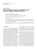
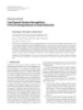
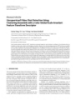
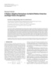
A Uniﬁed Low-Complexity Single-Band DS-CDMA UWB Receiver 467 0 0 NLMS µ = 1 −5 −5 −10 −10 MSE (dB) MSE (dB) RLS δ = 100 −15 −15 NLMS µ = 1 RLS δ = 100 −20 −20 LMMSE LMMSE −25 −25 −30 −30 0.2 0.4 0.6 0.8 0.2 0.4 0.6 0.8 0 1 0 1 Iteration normalized to ﬁlter length Iteration normalized to ﬁlter length (a) (b) Figure 1: Convergence of the receiver (Nc = 15, ψ = 1, SNR = 20 dB). (a) K = 1 and (b) K = 15. intractable to average out the entire channel and that this RLS when increasing the window length, as its knowledge of number of channels drawn from the model produces results the estimated inverse covariance matrix grows with the win- being within ±0.5 dB of the results obtained by performing dow length. the much larger number of simulations needed to average out the channel distribution. 6.2. BER simulations For NLMS, a step-size of µ = 1 was selected, as a smaller A series of Monte Carlo simulations have been performed step-size will produce unacceptable slow convergence. In the to estimate the BER performance of the receiver under the case of RLS, the value δ = 100 was chosen to minimize the assumption that the receiver has knowledge of the timing eﬀect of regularization as it is of higher importance not to parameter τ (1) . The number of iterations performed is kept constrain the adaptation when many users are active in the ﬁxed at Nite = Nfull and a total of 100 bit errors must occur UWB multipath channel. before a BER value is accepted. For a more in-depth description of the eﬀects of these From Figure 3 it can be seen that under both light- and adaptation parameters on the performance of the system in full-load conditions of 1 and 15 users, respectively, the RLS both the AWGN and UWB multipath channel, the interested algorithm is capable of providing reasonably good perfor- reader is referred to [13]. mance even in the case of restricting the ﬁlter length to ap- proximately ψ = 0.2. In the case of only a single user, the RLS 6.1. Convergence algorithm comes very close to the LMMSE receiver, but it is The convergence behavior of the receiver is important in or- not quite capable of reaching the bound when the load is in- der to determine the number of training bits necessary and creased to 15 users. The NLMS algorithm has been left out, verify that the ﬁlter coeﬃcients converge to the LMMSE so- as its general performance is unsatisfying [13], which is also lution. clear from the slow convergence depicted in Figure 1. Observing the convergence plotted in Figure 1, it should be noted how the addition of users makes the receiver con- 6.3. Synchronization verge more slowly as the dimension of the problem scales By inserting the needed parameters in (40), the ﬁlter length with the number of users. In the case of 15 users using the can be seen to increase by ψb = 0.048 in order to let the ﬁlter NLMS adaptation, the speed of convergence becomes very span an extra bit length. Focusing on the case of ψ = 0.2 slow and does not reach convergence within the simulated this results in ψ = 0.248 leading to L1 = 20 and L2 = 5. iterations. The RLS algorithm manages to converge much The BER performance of the receiver with this extended ﬁlter faster as a result of its knowledge of the estimated inverse length is plotted in Figure 3 under the assumption of being covariance matrix, but increasing the number of users also synchronized with the desired user. impacts it. The performance of the joint synchronization and de- In Figure 2a, the convergence of the WNLS algorithm is tection is shown in Figure 4 assuming Nd = 500. Further, plotted showing how the performance scales from NLMS to
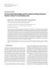
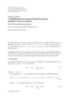
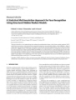
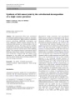
468 EURASIP Journal on Applied Signal Processing 5 1 −L2 0 0 −5 −1 Average MSE (dB) −10 MSE (dB) −2 −15 −3 −20 L1 LMMSE −4 −25 −30 −5 0.2 0.4 0.6 0.8 0 1 −10 −5 0 5 10 15 20 25 Iteration normalized to ﬁlter length es (bits) WNLS D = 16 WNLS D = 4056 (b) WNLS D = 64 NLMS µ = 1 WNLS D = 256 RLS δ = 100 WNLS D = 1024 (a) Figure 2: Convergence of the WNLS algorithm and the average MSE as a function of synchronization error (Nc = 15, ψ = 0.248, δ = 100). (a) K = 15, SNR = 20 dB and (b) K = 1, SNR = 10 dB, Nite = Nt = 127. 100 100 10−1 10−1 10−2 10−2 BER BER 10−3 10−3 10−4 10−4 10−5 10−5 10−6 10−6 −15 −10 −5 −15 −10 −5 0 5 10 15 20 0 5 10 15 20 SNR (dB) SNR (dB) ψ = 0.248 ψ = 0.248 AWGN AWGN ψ = 0.1 ψ = 0.5 ψ = 0.1 ψ = 0.5 ψ = 0.2 ψ = 0.2 LMMSE ψ = 0.2 ψ = 0.2 LMMSE (a) (b) Figure 3: The BER in the UWB multipath channel when the receiver is synchronized to the desired user (Nc = 15, Nite = Nfull = 4056, RLS δ = 100). (a) K = 1 and (b) K = 15.
A Uniﬁed Low-Complexity Single-Band DS-CDMA UWB Receiver 469 100 100 10−1 10−1 BER BER 10−2 10−2 10−3 10−3 −15 −10 −5 −15 −10 −5 0 5 10 15 20 0 5 10 15 20 SNR (dB) SNR (dB) K =4 K =4 AWGN AWGN K =1 K =8 K =1 K =8 K =2 K = 15 K =2 K = 15 (a) (b) Figure 4: Performance of the presented joint synchronization and detection scheme using the NLS algorithm (Nc = 15, ψ = 0.248, δ = 100). (a) Nite = Nt = 127 and (b) Nite = Nt = 255. Figure 2b plots the average MSE as a function of the ACKNOWLEDGMENTS synchronization error showing how on average the syn- The author would like to thank the anonymous reviewers for chronization error is minimized by (41). However, the syn- pointing out that the synchronization scheme was already in chronization error may be nonzero and the performance of existence, as the author was unaware of this fact. Further, the the receiver therefore degrades, as the captured energy be- author wishes to thank Thomas Fabricius, Spectronic Den- comes less. This, along with the fact that in the two cases mark, and Associate Professor Jan Larsen, Technical Univer- shown only Nite = 127 and Nite = 255 iterations are per- sity of Denmark, for their various fruitful discussions. In formed, explains why the BER in Figure 4 degrades com- addition, the author greatly appreciates the careful proof- pared to that of Figure 3, especially when more users are reading by Pedro Højen-Sørensen, Nokia Denmark, and Ole added. This performance degradation is the price paid by Nørklit, Nokia Denmark. using this low-complexity type of joint synchronization and detection. However, the achieved performance is the same as REFERENCES could be reached by using the RLS algorithm, but in the ex- [1] Federal Communications Commission (FCC), “Revision of ample where Nite = 127, the NLS algorithm lowers the com- part 15 of the commission’s rules regarding ultra-wideband plexity by a factor of G(Nite ) 10 resulting in approximately transmission systems,” First Report and Order, ET Docket 20 times the overall complexity reduction. 98-153, FCC 02-48; Adopted: February 2002; Released: April 2002. [2] A. Muqaibel, A. Safaai-Jazi, B. Woerner, and S. Riad, “UWB 7. CONCLUSION channel impulse response characterization using deconvolu- tion techniques,” in Proc. 45th IEEE Midwest Symposium A method for performing joint synchronization, channel on Circuits and Systems (MWSCAS ’02), vol. 3, pp. 605–608, estimation, and multiuser detection for single-band DS- Tulsa, Okla, USA, August 2002. CDMA UWB communications has been presented based on [3] U. Madhow, “Adaptive interference suppression for joint ac- quisition and demodulation of direct-sequence CDMA sig- the principles in [3, 8]. Simulations of the receiver show good nals,” in Proc. IEEE Military Communications Conference results in the UWB multipath channel in [9] using RLS adap- (MILCOM ’95), vol. 3, pp. 1200–1204, San Diego, Calif, USA, tation, but the complexity of the RLS adaptation is very high. November 1995. To help alleviate this problem, a novel algorithm termed the [4] U. Madhow, “MMSE interference suppression for timing ac- WNLS algorithm is derived, potentially lowering the compu- quisition and demodulation in direct-sequence CDMA sys- tational complexity while preserving the performance of the tems,” IEEE Trans. Commun., vol. 46, no. 8, pp. 1065–1075, RLS algorithm. 1998.
470 EURASIP Journal on Applied Signal Processing [5] R. Smith and S. Miller, “Acquisition performance of an adap- tive receiver for DS-CDMA,” IEEE Trans. Commun., vol. 47, no. 9, pp. 1416–1424, 1999. [6] M. Latva-aho, J. Lilleberg, J. Iinatti, and M. Juntti, “CDMA downlink code acquisition performance in frequency- selective fading channels,” in Proc. 9th IEEE International Symposium on Personal, Indoor and Mobile Radio Commu- nications (PIMRC ’98), vol. 3, pp. 1476–1480, Boston, Mass, USA, September 1998. [7] M. El-Tarhuni and A. Sheikh, “Performance analysis for an adaptive ﬁlter code-tracking technique in direct-sequence spread-spectrum systems,” IEEE Trans. Commun., vol. 46, no. 8, pp. 1058–1064, 1998. [8] Q. Li and L. A. Rusch, “Multiuser detection for DS-CDMA UWB in the home environment,” IEEE J. Select. Areas Com- mun., vol. 20, no. 9, pp. 1701–1711, 2002. [9] D. Cassioli, M. Z. Win, and A. F. Molisch, “The ultra-wide bandwidth indoor channel: from statistical model to simula- tions,” IEEE J. Select. Areas Commun., vol. 20, no. 6, pp. 1247– 1257, 2002. [10] M. Z. Win and R. A. Scholtz, “Impulse radio: how it works,” IEEE Commun. Lett., vol. 2, no. 2, pp. 36–38, 1998. [11] H. V. Poor and S. Verdu, “Probability of error in MMSE mul- tiuser detection,” IEEE Trans. Inform. Theory, vol. 43, no. 3, pp. 858–871, 1997. [12] S. Haykin, Adaptive Filter Theory, Prentice-Hall, Upper Sad- dle River, NJ, USA, 3rd edition, 1996. [13] L. P. B. Christensen, “Signal processing for ultra-wideband systems,” M.S. thesis, Informatics and Mathematical Mod- elling, Technical University of Denmark, Lyngby, Denmark, May 2003, http://www.imm.dtu.dk/∼lc. Lars P. B. Christensen was born in Copen- hagen, Denmark, in November 1978. He re- ceived the M.S.E.E. degree from the Tech- nical University of Denmark in May 2003, where he is currently working towards the Ph.D. degree. His current research interests are in the areas of digital communications and statistical signal processing.