Báo cáo hóa học: " Analysis of the Spatial Distribution of Galaxies by Multiscale Methods"

Chia sẻ: Linh Ha | Ngày: | Loại File: PDF | Số trang:15

Thêm vào BST

Báo xấu

35
lượt xem 3
download

Download Vui lòng tải xuống để xem tài liệu đầy đủ

Tuyển tập báo cáo các nghiên cứu khoa học quốc tế ngành hóa học dành cho các bạn yêu hóa học tham khảo đề tài: Analysis of the Spatial Distribution of Galaxies by Multiscale Methods

Chủ đề:

Bình luận(0) Đăng nhập để gửi bình luận!

Lưu

Nội dung Text: Báo cáo hóa học: " Analysis of the Spatial Distribution of Galaxies by Multiscale Methods"

EURASIP Journal on Applied Signal Processing 2005:15, 2455–2469 c 2005 Hindawi Publishing Corporation Analysis of the Spatial Distribution of Galaxies by Multiscale Methods J-L. Starck DAPNIA/SEDI-SAP, Service d’Astrophysique, CEA-Saclay, 91191 Gif-sur-Yvette, France Email: jstarck@cea.fr V. J. Mart´nez ı Observatori Astronomic de la Universitat de Val`ncia, Ediﬁci d’Instituts de Paterna, e ` Apartat de Correus 22085, 46071 Val`ncia, Spain e Email: vicent.martinez@uv.es D. L. Donoho Department of Statistics, Stanford University, Sequoia Hall, Stanford, CA 94305, USA Email: donoho@stanford.edu O. Levi Department of Statistics, Stanford University, Sequoia Hall, Stanford, CA 94305, USA Email: levio@bgumail.bgu.ac.il P. Querre DAPNIA/SEDI-SAP, Service d’Astrophysique, CEA-Saclay, 91191 Gif-sur-Yvette, France Email: philippe.querre@irsn.fr E. Saar Department of Cosmology, Tartu Observatory, Toravere 61602, Estonia Email: saar@aai.ee Received 17 June 2004; Revised 17 February 2005 Galaxies are arranged in interconnected walls and ﬁlaments forming a cosmic web encompassing huge, nearly empty, regions between the structures. Many statistical methods have been proposed in the past in order to describe the galaxy distribution and discriminate the diﬀerent cosmological models. We present in this paper multiscale geometric transforms sensitive to clusters, sheets, and walls: the 3D isotropic undecimated wavelet transform, the 3D ridgelet transform, and the 3D beamlet transform. We show that statistical properties of transform coeﬃcients measure in a coherent and statistically reliable way, the degree of clustering, ﬁlamentarity, sheetedness, and voidedness of a data set. Keywords and phrases: galaxy distribution, large-scale structures, wavelet, ridgelet, beamlet, multiscale methods. 1. INTRODUCTION descriptors. This could be the distribution of galaxies of a speciﬁc type in deep redshift surveys of galaxies (or of clus- Galaxies are not uniformly distributed throughout the uni- ters of galaxies).1 In order to compare models of structure formation, the diﬀerent distribution of dark matter particles verse. Voids, ﬁlaments, clusters, and walls of galaxies can be observed, and their distribution constrains our cosmologi- cal theories. Therefore we need reliable statistical methods 1 Making 3D maps of galaxies requires knowing how far away each galaxy to compare the observed galaxy distribution with theoretical is from Earth. One way to get this distance is to use Hubble’s law for the models and cosmological simulations. expansion of the universe and to measure the shift, called redshift, to redder The standard approach for testing models is to deﬁne colors of spectral features in the galaxy spectrum. The greater the redshift, a point process which can be characterized by statistical the larger the velocity, and, by Hubble’s law, the larger the distance.
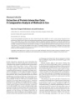
2456 EURASIP Journal on Applied Signal Processing in N-body simulations could be analyzed as well, with the 2. THE 3D WAVELET TRANSFORM same statistics. 2.1. The undecimated isotropic wavelet transform The two-point correlation function ξ (r ) has been the pri- For each a > 0, b1 , b2 , b3 ∈ R3 , the wavelet is deﬁned by mary tool for quantifying large-scale cosmic structure [1]. Assuming that the galaxy distribution in the Universe is a realization of a stationary and isotropic random process, ψa,b1 ,b2 ,b3 : R3 −→ R, the two-point correlation function can be deﬁned from the x1 − b1 x2 − b2 x3 − b3 probability δP of ﬁnding an object within a volume ele- ψa,b1 ,b2 ,b3 x1 , x2 , x3 = a−3/2 · ψ . , , ment δV at distance r from a randomly chosen object or a a a (1) position inside the volume: δP = n(1 + ξ (r ))δV , where n is the mean density of objects. The function ξ (r ) mea- Given a function f ∈ L2 (R3 ), we deﬁne its wavelet coef- sures the clustering properties of objects in a given vol- ﬁcients by ume. It is zero for a uniform random distribution, pos- itive (resp., negative) for a more (resp., less) clustered W f : R4 −→ R, distribution. For a hierarchical clustering or fractal pro- (2) cess, 1 + ξ (r ) follows a power-law behavior with exponent W f a, b1 , b2 , b3 = D2 − 3. Since ξ (r ) ∼ r −γ for the observed galaxy dis- ψ a,b1 ,b2 ,b3 (x) f (x)d x. tribution, the correlation dimension for the range where 3 − γ. The Fourier transform of ξ (r ) 1 is D2 Figure 1 shows an example of 3D wavelet function. the correlation function is the power spectrum. The di- It is standard to digitize the transform for data c(x, y , z) rect measurement of the power spectrum from redshift sur- with x, y , z ∈ {1, . . . , N } as follows. The wavelet transform veys is of major interest because model predictions are of a signal produces, at each scale j , a set of zero-mean coef- made in terms of the power spectral density. It seems clear ﬁcient values {w j }. Let φ be a lowpass ﬁlter and we deﬁne that the real space power spectrum departs from a sin- φ j (x) = φ(2 j x) and c j = c ∗ φ j . Using an undecimated gle power-law ruling out simple unbounded fractal mod- isotropic wavelet decomposition [23], the set {w j } has the els [2]. The two-point correlation function can been gen- same number of pixels as the signal and this wavelet trans- eralized to the N-point correlation function [3, 4], and form is redundant. Furthermore, using a wavelet deﬁned as all the hierarchy can be related with the physics responsi- the diﬀerence between the scaling functions of two successive ble for the clustering of matter. Nevertheless they are diﬃ- scales cult to measure, and therefore other related statistical mea- sures have been introduced as a complement in the sta- 1 xyz 1 xyz tistical description of the spatial distribution of galaxies = φ (x , y , z ) − φ , , ψ ,, , (3) 8 222 8 222 [5], such as the void probability function [6], the mul- tifractal approach [7], the minimal spanning tree [8, 9, 10], the Minkowski functionals [11, 12], or the J func- the original cube c = c0 can be expressed as the sum of all the tion [13, 14] which is deﬁned as the ratio J (r ) = (1 − wavelet scales and the smoothed array cJ : G(r ))/ (1 − F (r )), where F is the distribution function of the distance r of an arbitrary point in R3 to the near- J est object in the catalog, and G is the distribution func- c0,x, y,z = cJ ,x, y,z + w j ,x, y,z . (4) tion of the distance r of an object to the nearest ob- j =1 ject. Wavelets have also been used for analyzing the pro- jected 2D or the 3D galaxy distribution [15, 16, 17, 18, The set w = {w1 , w2 , . . . , wJ , cJ } represents the wavelet trans- 19]. form of the data. If we let W denote the wavelet transform New geometric multiscale methods have recently operator and N the pixels in c, the wavelet transform w emerged, the beamlet transform [20, 21] and the ridgelet (w = W c) has (J + 1)N pixels, for a redundancy factor of transform [22]; these allow us to represent data containing, J + 1. The scaling function φ is generally chosen as a spline respectively, ﬁlaments and sheets, while wavelets represent of degree 3, and the 3D implementation is based on three 1D well isotropic features (i.e., clusters in 3D). As each of these sets of (separable) convolutions. Like the scaling function φ, three transforms is tuned to a speciﬁc kind of feature, all of the wavelet function ψ is isotropic (see Figure 2). More de- them are useful and should be combined to describe a given tails can be found in [23, 24]. catalog. Sections 2, 3, and 4 describe, respectively, the 3D wavelet 3. THE 3D RIDGELET TRANSFORM transform, the 3D ridgelet transform, and the 3D beam- let transform. It is shown in Section 5 through a set of ex- 3.1. The 2D ridgelet transform periments how these three 3D transforms can be combined The 2d continuous ridgelet transform of a function f ∈ in order to describe statistically the distribution of galax- L2 (R2 ) was deﬁned in [22] as follows. ies.
Analysis of the Spatial Distribution of Galaxies 2457 1 1 0.5 0.5 0 0 −0.5 −0.5 −10 −5 −10 −5 0 5 10 0 5 10 −10 −10 −5 −5 0 0 60 5 5 50 10 10 40 −10 −5 −10 −5 0 5 10 0 5 10 30 20 10 60 50 40 50 60 30 y 30 40 20 10 10 20 x 00 Figure 1: Example of wavelet function. x3 (θ1 , θ2 ) line θ1 line θ2 θ1 x1 x1 θ1 x2 x2 (a) (b) Figure 2: Deﬁnition of angle1 θ1 and θ2 in (a) R2 (2D case) and (b) R3 (3D case). Given a function f ∈ L2 (R2 ), we deﬁne its ridgelet coeﬃ- Select a smooth function ψ ∈ L2 (R), satisfying admissi- bility condition cients by 2 R f : R3 −→ R, ˆ ψ (ξ ) dξ < ∞, (5) |ξ | (7) R f a, b, θ1 = ψ a,b,θ1 (x) f (x)d x. which holds if ψ has a suﬃcient decay and a vanishing mean ψ (t )dt = 0 (ψ can be normalized so that it has unit energy It has been shown [22] that the ridgelet transform is pre- 1/ (2π ) |ψ (ξ )|2 dξ = 1). For each a > 0, b ∈ R, and θ1 ∈ ˆ cisely the application of a 1D wavelet transform to the slices [0, 2π [, we deﬁne the ridgelet by of the Radon transform (where the angular variable θ1 is con- stant). This method is in a sense optimal to detect lines of ψa,b,θ1 : R2 −→ R, the size of the image (the integration increase as the length of x1 cos θ1 + x2 sin θ1 − b (6) the line). More details on the implementation of the digital ψa,b,θ1 x1 , x2 = a−1/2 · ψ . ridgelet transform can be found in [25]. a
2458 EURASIP Journal on Applied Signal Processing 1 0.8 0.6 0.4 0.2 0 −0.2 −2 0 2 (b) (a) Figure 3: Example of 2D ridgelet function. ˆ (1) 3D-FFT. Compute c(k1 , k2 , k3 ), the 3D FFT of the cube c(i1 , i2 , i3 ). (2) Cartesian-to-spherical conversion. Using an interpolation ˆ scheme, substitute the sampled values of c obtained on 0.4 the Cartesian coordinate system (k1 , k2 , k3 ) with sampled values in a spherical coordinate system (θ1 , θ2 , ρ). 2 (3) Extract lines. Extract the 3N 2 lines (of size N ) passing 0.2 1 ˆ through the origin and the boundary of c. 0 0 (4) 1D-IFFT. Compute the 1D inverse FFT on each line. −1 (5) 1D-WT. Compute the 1D wavelet transform on each −0.2 −2 60 line. 50 40 Algorithm 1: The 3D ridgelet transform algorithm. 30 20 where a > 0, b ∈ R, θ1 ∈ [0, 2π [, and θ2 ∈ [0, π [. The 10 ridgelet function is deﬁned by 60 50 40 ψa,b,θ1 ,θ2 : R3 −→ R, 60 30 40 50 20 y 20 30 10 ψa,b,θ1 ,θ2 x1 , x2 , x3 10 00 x x1 cos θ1 cos θ2 + x2 sin θ1 cos θ2 + x3 sin θ2 − b = a−1/2 · ψ . Figure 4: Example of ridgelet function. a (9) Figure 4 shows an example of ridgelet function. It is a Figure 3 (left) shows an example ridgelet function. This wavelet function in the direction deﬁned by the line (θ1 , θ2 ), function is constant along lines x1 cos θ + x2 sin θ = const. and it is constant along the orthogonal plane to this line. Transverse to these ridges it is a wavelet (see Figure 3(b)). As in the 2D case, the 3D ridgelet transform can be built by extracting lines in the Fourier domain. Let c(i1 , i2 , i3 ) be a 3.2. From 2D to 3D cube of size (N , N , N ); the steps can be seen in Algorithm 1 steps. The 3D continuous ridgelet transform of a function f ∈ Figure 5 shows the 3D ridgelet transform ﬂowgraph. The L2 (R3 ) is given by 3D ridgelet transform allows us to detect sheets in a cube. R f : R4 −→ R, Local 3D ridgelet transform The ridgelet transform is optimal to ﬁnd sheets of the size (8) R f a, b, θ1 , θ2 = of the cube. To detect smaller sheets, a partitioning must be ψ a,b,θ1 ,θ2 (x) f (x)dx,
Analysis of the Spatial Distribution of Galaxies 2459 Euclidian space Fourier space x3 kx3 (θ1 , θ2 ) line 1D wavelet transform 1D WT ρ of (θ1 , θ2 ) line (θ1 , θ2 ) line θ2 Scale j +1 kx1 Plane ⊥ (θ1 , θ2 ) line Plane ⊥ (θ1 , θ2 ) line, x1 Scale j Spatial radius ρ scale j θ1 Scale 1 x2 kx2 Lines Lines Radon transform 1D wavelet transform Figure 5: 3D ridgelet transform ﬂowgraph. introduced [26]. The cube c is decomposed into blocks of since any algorithm based on this set will have a complexity lower side-length b so that for a N × N × N cube, we count with lower bound of n6 and hence be unworkable for typical N/b blocks in each direction. After the block partitioning, the 3D data size. tranform is tuned for sheets of size b × b and of thickness a j , a j corresponding to the diﬀerent dyadic scales used in the 4.2. The beamlet system transformation. A dyadic cube C (k1 , k2 , k3 , j ) ⊂ [0, 1]3 is the collection of 3D points 4. THE 3D BEAMLET TRANSFORM 4.1. Deﬁnition k1 k1 + 1 k2 (k2 + 1) × x1 , x2 , x3 : , , 2j 2j 2j 2j The X-ray transform of a continuum function f (x, y , z) with (x, y , z) ∈ R3 is deﬁned by (11) k3 k3 + 1 × , , 2j 2j (X f )(L) = f ( p )d p , (10) where 0 ≤ k1 , k2 , k3 < 2 j for an integer j ≥ 0, called the scale. L Such cubes can be viewed as descended from the unit cube C (0, 0, 0, 0) = [0, 1]3 by recursive partitioning. Hence, where L is a line in R3 , and p is a variable indexing points in the result of splitting C (0, 0, 0, 0) in half along each axis is the the line. The transformation contains all line integrals of f . eight cubes C (k1 , k2 , k3 , 1) where ki ∈ {0, 1} (see Figure 6), The beamlet transform (BT) can be seen as a multiscale digi- splitting those in half along each axis we get the 64 subcubes tal X-ray transform. It is multiscale transform because, in ad- C (k1 , k2 , k3 , 2) where ki ∈ {0, 1, 2, 3}, and if we decompose dition to the multiorientation and multilocation line integral the unit cube into n3 voxels using a uniform n-by-n-by-n grid calculation, it integrated also over line segments at diﬀerent with n = 2J dyadic, then the individual voxels are the n3 cells lengths. The 3D BT is an extension to the 2D BT, proposed C (k1 , k2 , k3 , J ), 0 ≤ k1 , k2 , k3 < n. by Donoho and Huo [20]. Associated to each dyadic cube we can build a system of line segments that have both of their end-points lying on the The system of 3D beams cube boundary. We call each such segment a beamlet. If we The transform requires an expressive set of line segments, consider all pairs of boundary voxel corners, we get O(n4 ) including line segments with various lengths, locations, and beamlets for a dyadic cube with a side-length of n voxels (we actually work with a slightly diﬀerent system in which orientations lying inside a 3D volume. A seemingly natural candidate for the set of line segments each line is parametrized by a slope and an intercept instead is the family of all line segments between each voxel corner of its end-points as explained below). However, we will still have O(n4 ) cardinality. Assuming a voxel size of 1/n we get and every other voxel corner, the set of 3D beams. For a 3D data set with n3 voxels, there are O(n6 ) 3D beams. It is infeasi- J + 1 scales of dyadic cubes where n = 2J , for any scale 0 ≤ j ≤ J there are 23 j dyadic cubes of scale j and since each ble to use the collection of 3D beams as a basic data structure
2460 EURASIP Journal on Applied Signal Processing C (1, 1, 1, 1) C (0, 0, 0, 0) 1 1 C (0, 1, 1, 1) 0.5 C (1, 0, 1, 1) 0.5 C (0, 1, 0, 1) 0 C (1, 0, 0, 1) 1 0 1 0.5 1 0.5 0.5 1 00 0.5 00 C (0, 1, 0, 1) (a) (b) Figure 6: Dyadic cubes. (a) (b) Figure 7: Examples of beamlets at two diﬀerent scales: (a) scale 0 (coarsest scale) and (b) scale 1 (next ﬁner scale). dyadic cube at scale j has a side-length of 2J − j voxels, we get The slopes and intercepts run through equispaced sets: O(24(J − j ) ) beamlets associated with the dyadic cube and a to- tal of O(24J − j ) = O(n4 / 2 j ) beamlets at scale j . If we sum the n n 2 number of beamlets at all scales we get O(n4 ) beamlets. sx , s y , sz ∈ : = − ,..., , 2−1 n 2 This gives a multiscale arrangement of line segments in (13) 3D with controlled cardinality of O(n4 ), the scale of a beam- n n tx , t y , tz ∈ : − ,..., . let is deﬁned as the scale of the dyadic cube it belongs to 2−1 2 so lower scales correspond to longer line segments and ﬁner scales correspond to shorter line segments. Figure 7 shows 2 beamlets at diﬀerent scales. Beamlets in a data cube of side n have lengths between √ n/ 2 and 3n (the main diagonal). To index the beamlets in a given dyadic cube, we use slope-intercept coordinates. For a data cube of n × n × n vox- els, consider a coordinate system with the cube center of mass Computational aspects at the origin and a unit length for a voxel. Hence, for (x, y , z) Beamlet coeﬃcients are line integrals over the set of beam- in the data cube we have |x|, | y |, |z| ≤ n/ 2. We can consider lets. A digital 3D image can be regarded as a 3D piece-wise three kinds of lines: x-driven, y -driven, and z-driven, depend- constant function and each line integral is just a weighted ing on which axis provides the shallowest slopes. An x-driven sum of the voxel intensities along the corresponding line seg- line takes the form ment. Donoho and Levi [21] discuss in detail diﬀerent ap- proaches for computing line integrals in a 3D digital image. Computing the beamlet coeﬃcients for real application data z = sz x + tz , y = sy x + ty (12) sets can be a challenging computational task since for a data cube with n × n × n voxels, we have to compute O(n4 ) co- eﬃcients. By developing eﬃcient cache aware algorithms we with slopes sz , s y , and intercepts tz and t y . Here the slopes |sz |, |s y | ≤ 1. y - and z-driven lines are deﬁned with an in- are able to handle 3D data sets of size up to n = 256 on a terchange of roles between x and y or z, as the case may be. typical desktop computer in less than a day running time.
Analysis of the Spatial Distribution of Galaxies 2461 1 ˆ (1) 3D-FFT. Compute c(k1 , k2 , k3 ), the three-dimensional 0.5 FFT of the cube c(i1 , i2 , i3 ). (2) Cartesian to spherical conversion. Using an interpolation 0 ˆ scheme, substitute the sampled values of c obtained on the Cartesian coordinate system (k1 , k2 , k3 ) with sampled −0.5 values in a spherical coordinate system (θ1 , θ2 , ρ). −10 −5 0 5 10 (3) Extract planes. Extract the 3N 2 planes (of size N × N ) −10 passing through the origin (each line used in the 3D −5 ridgelet transform deﬁnes a set of orthogonal planes; we 0 take the one including the origin). 60 (4) 2D-IFFT. Compute the 2D inverse FFT on each plane. 5 (5) 2D-WT. Compute the 2D wavelet transform on each 50 10 plane. 40 −10 −5 0 5 10 30 20 Algorithm 2: The 3D beamlet transform algorithm. 10 60 4.3. The FFT-based transformation 50 40 60 30 Let ψ ∈ L2 (R2 ) be a smooth function satisfying a 2D vari- 40 50 y 20 20 30 10 ant of the admissibility condition, the 3D continuous beamlet 10 00 x transform of a function f ∈ L2 (R3 ) is given by Figure 8: Example of beamlet function. B f : R5 −→ R, (14) We will mention that in many cases there is no interest in the B f a, b1 , b2 , θ1 , θ2 = ψ a,b,θ1 ,θ2 (x) f (x)d x, coarsest scales coeﬃcient that consumes most of the compu- tation time and in that case the overall running time can be signiﬁcantly faster. The algorithms can also be easily imple- where a > 0, b1 , b2 ∈ R, θ1 ∈ [0, 2π [, and θ2 ∈ [0, π [. The mented on a parallel machine of a computer cluster using a beamlet function is deﬁned by system such as MPI in order to solve bigger problems. ψa,b1 ,b2 ,θ1 ,θ2 : R3 −→ R, (15) − x1 sin θ1 + x2 cos θ1 + b1 x1 cos θ1 cos θ2 + x2 sin θ1 cos θ2 − x3 sin θ2 + b2 ψa,b1 ,b2 ,θ1 ,θ2 x1 , x2 , x3 = a−1/2 · ψ . , a a The Fourier transform of the m-dimensional partial Figure 8 shows an example of beamlet function. It is con- radon transform Radm f is related to the Fourier transform stant along lines of direction (θ1 , θ2 ), and a 2D wavelet func- of f (F f ) by the projection-slice relation tion along plane orthogonal to this direction. The 3D beamlet transform can be built using the “gen- Fn−m+1 Radm f k, km+1 , . . . , kn eralized projection-slice theorem” [27]. Let f (x) be a func- (16) tion on Rn ; and let Radm f denote the m-dimensional par- = {F f } k µm , km+1 , . . . , kn . tial Radon transform along the ﬁrst m directions, m < n. Radm f is a function of ( p, µm ; xm+1 , . . . , xn ), µm a unit di- Let c(i1 , i2 , i3 ) be a cube of size (N , N , N ); the steps of the rectional vector in Rn (note that for a given projection an- Beamlet algorithm can be seen in the following Algorithm 2. gle, the m-dimensional partial Radon transform of f (x) has Figure 9 gives the 3D beamlet transform ﬂowgraph. The (n−m) untransformated spatial dimensions and a (n−m+1)- 3D beamlet transform allows us to detect ﬁlaments in a cube. dimensional projection proﬁle). In addition, let {F f }(k) The beamlet transform algorithm presented in this section diﬀers from the one presented in [28]; see the discussion in denote the n-dimensional Fourier transform where x and k are conjugate variables. [21].
2462 EURASIP Journal on Applied Signal Processing 2D wavelet transform of (θ1 , θ2 ) line ⊥ plane Euclidian space Fourier space (θ1 , θ2 ) line ⊥ plane at position (ρ2 , ρ1 ) kx3 at position (ρ2 , ρ1 ) x3 and scale 1 Plane ⊥ (θ1 , θ2 ) line including origin (θ1 , θ2 ) line Scale 1 ρ2 2D y WT 2D xWT θ2 kx1 ρ1 x1 θ1 Scale j x2 kx2 Planes Planes Partial Radon transform 2D wavelet transform Figure 9: 3D beamlet transform ﬂowgraph. 5. EXPERIMENTS point in each of the vertices of a Voronoi tessellation of 1500 cells deﬁned by 1500 nuclei distributed follow- 5.1. Experiment 1 ing a binomial process. There are 10 085 vertices lying within a box of 141.4 h−1 Mpc side. We have simulated three data sets containing, respectively, a cluster, a plane, and a line. To each data set, Poisson noise (ii) The second point pattern represents the galaxy po- has been added with eight diﬀerent background levels. We sitions extracted from a cosmological Λ-CDM N- applied the three transforms on the 24 simulated data sets. body simulation. The simulation has been carried The coeﬃcient distribution from each transformation was out by the Virgo consortium and related groups (see normalized using twenty realizations of a Poisson noise hav- http://www.mpa-garching.mpg.de/Virgo). The simu- lation is a low-density (Ω = 0.3) model with cosmo- ing the same number of counts as in the data. logical constant Λ = 0.7. It is, therefore, an approxi- Figure 10 shows the maximum value of the normal- ized distribution versus the noise level for our three simu- mation to the real galaxy distribution [29]. There are 15 445 galaxies within a box with side 141.3 h−1 Mpc. lated data sets. As expected, wavelets, ridgelets, and beam- lets are, respectively, the best for detecting clusters, sheets, Galaxies in this catalog have stellar masses exceeding 2 × 1010 M . and lines. A feature can typically be detected with a very high signal-to-noise ratio in a matched transform, while re- Figure 11 shows the two simulated data sets, and maining indetectible in some other transforms. For exam- Figure 12 shows the two-point correlation function curve ple, the wall is detected at more than 60σ by the ridgelet for the two-point processes. The two-point ﬁelds are diﬀer- transform, but at less than 5σ by the wavelet transform. ent, but as can be seen in Figure 12, both have very similar The line is detected almost at 10σ by the beamlet trans- two-point correlation functions in a huge range of scales (2 form, and with worse than 3σ detection level by wavelets. decades). These results show the importance of using several trans- We have applied the three transforms to each data set, forms for an optimal detection of all features contained in j jj and we have calculated the skewness vector S = (sw , sr , sb ) a data set. j j j and the kurtosis vector K = (kw , kr , kb ) at each scale j . 5.2. Experiment 2 j jj sw , sr , sb are, respectively, the skewness at scale j of the wavelet coeﬃcients, the ridgelet coeﬃcients, and the beamlet coeﬃ- We use here two simulated data sets to illustrate the discrim- inative power of multiscale methods. The ﬁrst one is a sim- j j j cients. kw , kr , kb are, respectively, the kurtosis at scale j of the ulation from stochastic geometry. It is based on a Voronoi wavelet coeﬃcients, the ridgelet coeﬃcients, and the beamlet model. The second one is a mock catalog of the galaxy distri- coeﬃcients. Figure 13 shows the kurtosis and the skewness bution drawn from a Λ-CDM N-body cosmological model vectors of the two data sets at the two ﬁrst scales. In contrast [29]. Both processes have very similar two-point correlation to the case with the two-point correlation function, this ﬁg- functions at small scales, although they look quite diﬀerent ure shows strong diﬀerences between the two data sets, par- and have been generated following completely diﬀerent al- ticularly on the wavelet axis, which indicates that the second gorithms. data contains more or higher density clusters than the ﬁrst (i) The ﬁrst comes from Voronoi simulation. We locate a one.
Analysis of the Spatial Distribution of Galaxies 2463 30 Normalized maximum value 25 3 20 2.5 15 10 2 5 1.5 0 30 25 1 20 25 30 1510 0.01 0.1 1 15 20 5 5 10 Noise level 00 Wavelet Ridgelet Beamlet (a) 30 Normalized maximum value 60 25 50 20 40 15 30 10 5 20 0 10 30 25 20 25 30 15 0.01 0.1 1 10 5 15 20 0 0 5 10 Noise level Wavelet Ridgelet Beamlet (b) 30 Normalized maximum value 25 8 20 6 15 10 4 5 0 2 30 25 20 0.01 0.1 25 30 1 15 10 5 15 20 0 0 5 10 Noise level Wavelet Ridgelet Beamlet (c) Figure 10: Poisson realization for a low noise level: simulation of cubes containing (a) a cluster , (b) a plane, and (c) a line.
2464 EURASIP Journal on Applied Signal Processing 140 140 120 120 100 100 80 80 60 60 40 40 20 20 140 140 120 120 100 80 100 80 120 140 120 140 60 60 80 100 80 100 40 40 60 60 20 20 20 40 20 40 (a) (b) (c) (d) Figure 11: Simulated data sets. (a) The Voronoi vertices point pattern and (b) the galaxies of the GIF Λ-CDM N-body simulation. (c) One 10 h−1 width slice of each data set. 100 000 5.3. Experiment 3 In this experiment, we have used a Λ-CDM simulation based 10 000 on the N-body hydrodynamical code, RAMSES [30]. The simulation uses an adaptive mesh reﬁnement (AMR) tech- nique, with a tree-based data structure allowing recursive 1000 grid reﬁnements on a cell-by-cell basis. The simulated data were obtained using 2563 particles and 4.1 × 107 cells in the ξ (r ) 100 AMR grid, reaching a formal resolution of 81923 . The box size was set to 100h−1 Mpc, with the following cosmological parameters: 10 Ωm = 0.3, Ωλ = 0.7, Ωb = 0.039, 1 (17) h = 0.7, σ8 = 0.92. 0.1 0.01 0.1 1 10 We used the results of this simulation at six diﬀerent r redshifts (z = 5, 3, 2, 1, 0.5, 0). Figure 14 shows a projec- Voronoi tion of the simulated cubes along one axis. We applied the Λ-CDM (GIF) 3D wavelet transform, the 3D beamlet transform, and the 2 2 3D ridgelet transform on the six data sets. Let σW ,z, j , σR,z, j , Figure 12: The two-point correlation function of the Voronoi ver- 2 tices process and the GIF Λ-CDM N-body simulation. They are very σB,z, j denote the variance of the wavelet, the ridgelet, and the beamlet coeﬃcients of the scale j at redshift z. similar in the range [0.02, 2] h−1 Mpc.
Analysis of the Spatial Distribution of Galaxies 2465 3 6 2.5 5 2 Wavelet Wavelet 4 1.5 3 1 2 0.5 1 0 0 4.6 5.7 3.8 3 4.3 5.5 Rid Rid 1.5 1.9 2.9 3.6 gel gel 1.4 1.8 00 00 et et eamlet eamlet B B Simulated ﬁle 1 Simulated ﬁle 1 Simulated ﬁle 2 Simulated ﬁle 2 (a) (b) 25 15 20 Wavelet Wavelet 15 10 10 5 5 0 0 10.8 6.4 4.3 7.2 18.8 17.5 Rid Rid 2.1 3.6 12.6 11.7 6.3 gel gel 5.8 00 00 et et t t Beamle Beamle Simulated ﬁle 1 Simulated ﬁle 1 Simulated ﬁle 2 Simulated ﬁle 2 (c) (d) Figure 13: Skewness and kurtosis for the two simulated data sets: (a) skewness, scale 1, (b) skewness, scale 2, (c) kurtosis, scale 1, and (d) kurtosis, scale 2. The Mw/b curve does not show much evolution, while the Figure 15, shows, respectively, from top to bottom, the 2 wavelet spectrum Pw (z, j ) = σW ,z, j , the beamlet spectrum Mw/r curve presents a signiﬁcant slope. This shows that the 2 Pb (z, j ) = σB,z, j , and the ridgelet spectrum Pr (z, j ) = beamlet transform is more sensitive to clustering than the ridgelet transform. This is not surprising since the support 2 σR,z, j . In order to see the evolution of matter distribution of beamlets is much smaller than the support of ridgelets. with redshift and scale, we calculate the ratio Mw/b ( j , z) = Mw/r increases with z, reﬂecting the cluster formation. The Pw (z, j )/Pb (z, j ) and Mw/r ( j , z) = Pw (z, j )/Pr (z, j ). combination of multiscale transformations gives clear in- Figure 16 shows the Mw/b and Mw/r curves as a function −1 −1 formation about the degree of clustering, ﬁlamentarity, and of z and Figure 17 shows the Mw/b and Mw/r curves as a func- sheetedness. tion of the scale number j .
2466 EURASIP Journal on Applied Signal Processing 2.2 × 107 4.6 × 104 Log (ratio) 1 × 102 2.2 × 10−1 0 2 4 Scale number z=5 z=1 z=3 z = 0.5 z=2 z=0 (a) 104 102 Log (ratio) 100 10−2 0 1 2 Figure 14: Λ-CDM simulation at diﬀerent redshifts. Scale number z=5 z=1 z=3 z = 0.5 z=2 z=0 6. CONCLUSION (b) We have introduced in this paper a new method to analyze catalogs of galaxies based on the distribution of coeﬃcients 105 obtained by several geometric multiscale transforms. We have introduced two new multiscale decompositions, the 3D ridgelet transform and the 3D beamlet transform, 103 matched to sheetlike and ﬁlament features, respectively. We Log (ratio) described fast implementations using FFTs. We showed that combining the information related to wavelet, ridgelet, and beamlet coeﬃcients leads to a new description of point cat- 101 alogs. In this paper, we described transform coeﬃcients us- ing skewness and kurtosis, but another recent statistic esti- mator such the higher criticism [31] could be used as well. 10−1 Each multiscale transform is very sensitive to one kind of fea- 0 1 2 ture: wavelets to clusters; beamlets to ﬁlaments; and ridgelets Scale number to walls. A similar method has been proposed for analyz- z=5 z=1 ing CMB maps [32] where both the curvelet and the wavelet z=3 z = 0.5 transforms were used for the detection and the discrimina- z=2 z=0 tion of non-Gaussianities. This combined multiscale statistic (c) is very powerful and we have shown that two data sets with identical two-point correlation functions are clearly distin- guished by our approach. These new tools lead to better con- Figure 15: (a) Wavelet spectrum, (b) beamlet spectrum, and (c) ridgelet spectrum at diﬀerent redshifts. straints on cosmological models.
Analysis of the Spatial Distribution of Galaxies 2467 4 1 0.63 3 Log (ratio) Ratio 0.4 2 0.25 0 1 2 1 Scale number 5 4 3 2 1 0 z z=5 z=1 z=3 z = 0.5 Scale 3 z=2 z=0 Scale 2 Scale 1 (a) (a) 0.933 6.31 3.98 0.667 Log (ratio) Ratio 2.51 0.4 1.58 0 1 2 0.133 5 4 3 2 1 0 Scale number z z=5 z=1 z=3 z = 0.5 Scale 3 z=2 z=0 Scale 2 Scale 1 (b) (b) Figure 17: (a) Beamlet/wavelet 1/Mw/b (z, j ) and (b) ridgelet/ Figure 16: (a) Wavelet/beamlet Mw/b (z, j ) and (b) wavelet/ridgelet wavelet 1/Mw/r (z, j ) curves at diﬀerent redshifts. Mw/r (z, j ) curves for the scale number j equal to 1,2, and 3. ACKNOWLEDGMENTS sky survey,” The Astrophysical Journal, vol. 606, no. 2, part 1, We wish to thank Romain Teyssier for giving us the Λ- pp. 702–740, 2004. [3] S. Szapudi and A. S. Szalay, “A new class of estimators for the CDM simulated data used in the third experiment. This work N-point correlations,” Astrophysical Journal Letters, vol. 494, has been supported by the Spanish MCyT project AYA2003- no. 1, pp. L41–L44, 1998. 08739-C02-01 (including FEDER), the Generalitat Valen- [4] P. J. E. Peebles, “The galaxy and mass N-point correlation ciana project GRUPOS03/170, the National Science Founda- functions: a blast from the past,” in Historical Development of tion Grant DMS-01-40587 (FRG), and the Estonian Science Modern Cosmology, V. J. Mart´nez, V. Trimble, and M. J. Pons- ı Foundation Grant 4695. Border´a, Eds., vol. 252 of ASP Conference Series, Astronomi- ı cal Society of the Paciﬁc, San Francisco, Calif, USA, 2001. V. J. Mart´nez and E. Saar, Statistics of the Galaxy Distribution, [5] ı REFERENCES Chapman & Hall/CRC press, Boca Raton, Fla, USA, 2002. [1] P. J. E. Peebles, The Large-Scale Structure of the Universe, [6] S. Maurogordato and M. Lachieze-Rey, “Void probabilities Princeton University Press, Princeton, NJ, USA, 1980. in the galaxy distribution—scaling and luminosity segrega- [2] M. Tegmark, M. R. Blanton, M. A. Strauss, et al., “The three- tion,” The Astrophysical Journal, vol. 320, pp. 13–25, Septem- dimensional power spectrum of galaxies from the sloan digital ber 1987.
2468 EURASIP Journal on Applied Signal Processing [7] V. J. Mart´nez, B. J. T. Jones, R. Dom´nguez-Tenreiro, and ı ı Data Analysis: The Multiscale Approach, Cambridge Univer- R. van de Weygaert, “Clustering paradigms and multifractal sity Press, Cambridge, UK, 1998. measures,” The Astrophysical Journal, vol. 357, no. 1, pp. 50– [24] J.-L. Starck and F. Murtagh, “Astronomical Image and Data 61, 1990. Analysis,” @#pages, Springer, Berlin, Germany, 2002. [8] S. P. Bhavsar and R. J. Splinter, “The superiority of the min- ` [25] J.-L. Starck, E. J. Candes, and D. L. Donoho, “The curvelet imal spanning tree in percolation analyses of cosmological transform for image denoising,” IEEE Trans. Image Processing, data sets,” Monthly Notices of the Royal Astronomical Society, vol. 11, no. 6, pp. 670–684, 2002. vol. 282, no. 4, pp. 1461–1466, 1996. ` [26] E. J. Candes, “Harmonic analysis of neural networks,” Applied [9] L. G. Krzewina and W. C. Saslaw, “Minimal spanning tree and Computational Harmonic Analysis, vol. 6, no. 2, pp. 197– statistics for the analysis of large-scale structure,” Monthly No- 218, 1999. tices of the Royal Astronomical Society, vol. 278, no. 3, pp. 869– [27] P. C. Lauterbur and Z.-O. Liang, Principle of Magnetic Reso- 876, 1996. nance Imaging, IEEE Press, New York, NY, USA, 2000. [10] A. G. Doroshkevich, D. L. Tucker, R. Fong, V. Turchaninov, D. L. Donoho, O. Levi, J.-L. Starck, and V. J. Mart´nez, “Multi- [28] ı and H. Lin, “Large-scale galaxy distribution in the Las Cam- scale geometric analysis for 3D catalogs,” in Astronomical Data panas Redshift Survey,” Monthly Notices of the Royal Astro- Analysis II, J.-L. Starck and F. Murtagh, Eds., vol. 4847 of Pro- nomical Society, vol. 322, no. 2, pp. 369–388, 2001. ceedings of SPIE, pp. 101–111, Waikoloa, Hawaii, USA, August [11] K. R. Mecke, T. Buchert, and H. Wagner, “Robust morpho- 2002. logical measures for large-scale structure in the universe,” As- G. Kauﬀmann, J. M. Colberg, A. Diaferio, and S. D. M. White, [29] tronomy & Astrophysics, vol. 288, no. 3, pp. 697–704, 1994. “Clustering of galaxies in a hierarchical universe—I. Methods [12] M. Kerscher, “Statistical analysis of large-scale structure in the and results at z = 0,” Monthly Notices of the Royal Astronomical universe,” in Statistical Physics and Spatial Statistics: The Art of Society, vol. 303, no. 1, pp. 188–206, 1999. Analyzing and Modeling Spatial Structures and Pattern Forma- [30] R. Teyssier, “Cosmological hydrodynamics with adaptive tion, K. Mecke and D. Stoyan, Eds., vol. 554 of Lecture Notes mesh reﬁnement—A new high resolution code called RAM- in Physics, pp. 36–71, Springer, Berlin, Germany, 2000. SES,” Astronomy & Astrophysics, vol. 385, no. 1, pp. 337–364, [13] M. N. M. Van Lieshout and A. J. Baddeley, “A nonparamet- 2002. ric measure of spatial interaction in point patterns,” Statistica [31] D. L. Donoho and J. Jin, “Higher criticism for detecting sparse Neerlandica, vol. 50, no. 3, pp. 344–361, 1996. heterogeneous mixtures,” Tech. Rep., Statistics Department, [14] M. Kerscher, M. J. Pons-Border´a, J. Schmalzing, et al., “A ı Stanford University, Stanford, Calif, USA, 2002. global descriptor of spatial pattern interaction in the galaxy [32] J.-L. Starck, N. Aghanim, and O. Forni, “Detection and distribution,” The Astrophysical Journal, vol. 513, no. 2, part 1, discrimination of cosmological non-Gaussian signatures by pp. 543–548, 1999. multi-scale methods,” Astronomy & Astrophysics, vol. 416, [15] E. Escalera, E. Slezak, and A. Mazure, “New evidence for no. 1, pp. 9–17, 2004. subclustering in the Coma cluster using the wavelet analy- sis,” Astronomy & Astrophysics, vol. 264, no. 2, pp. 379–384, 1992. J-L. Starck has a Ph.D. degree from the [16] E. Slezak, V. de Lapparent, and A. Bijaoui, “Objective detec- University Nice-Sophia Antipolis and a Ha- tion of voids and high-density structures in the ﬁrst CfA red- bilitation degree from the University Paris shift survey slice,” The Astrophysical Journal, vol. 409, no. 2, XI. He was a Visitor at the European pp. 517–529, 1993. Southern Observatory (ESO) in 1993, at [17] V. J. Mart´nez, S. Paredes, and E. Saar, “Wavelet analysis of the ı multifractal character of the galaxy distribution,” Monthly No- UCLA in 2004, and at the Statistics De- tices of the Royal Astronomical Society, vol. 260, no. 2, pp. 365– partment, Stanford University, in 2000 and 375, 1993. 2005. He has been a researcher at the service [18] A. Pagliaro, V. Antonuccio-Delogu, U. Becciani, and M. Gam- d’Astrophysique, CEA-sacloy, since 1994. bera, “Substructure recovery by three-dimensional discrete His research interests include image pro- wavelet transforms,” Monthly Notices of the Royal Astronom- cessing, statistical methods in astrophysics, and cosmology. He is ical Society, vol. 310, no. 3, pp. 835–841, 1999. also author of two books entitled Image Processing and Data Analy- [19] T. Kurokawa, M. Morikawa, and H. Mouri, “Scaling analysis sis: the Multiscale Approach, and Astronomical Image and Data Anal- of galaxy distribution in the Las Campanas Redshift Survey ysis. data,” Astronomy & Astrophysics, vol. 370, no. 2, pp. 358–364, 2001. V. J. Mart´nez received his Ph.D. degree in ı [20] D. L. Donoho and X. Huo, “Beamlets and multiscale image mathematics from the University of Valen- analysis,” in Multiscale and Multiresolution Methods, vol. 20 of cia in 1989, after preparing his thesis at Lecture Notes in Computational Science and Engineering, pp. NORDITA, Copenhagen, where his Adviser 149–196, Springer, New York, NY, USA, 2001. was Bernard Jones. In 1991, he got a perma- [21] D. L. Donoho and O. Levi, “Fast x-ray and beamlet trans- nent position at the University of Valencia forms for three-dimensional data,” in Modern Signal Process- as an Associate Professor in astronomy and ing, D. Rockmore and D. Healy, Eds., vol. 46 of Mathematical astrophysics. He is currently the Director of Science Research Institute Publications, Cambridge University ´ the Observatori Astronomic dela Universi- Press, Cambridge, UK, March 2002. tat de Valencia. He works on the statistical ` [22] E. J. Candes and D. L. Donoho, “Ridgelets: the key to high properties of the large-scale structure of the Universe. He is also dimensional intermittency?” Philosophical Transactions of the involved in observational projects to study the mass and extent of Royal Society of London A, vol. 357, pp. 2495–2509, September dark halos around elliptical galaxies. He is the coauthor, with E. 1999. Saar, of the book Statistics of the Galaxy Distribution. [23] J.-L. Starck, F. Murtagh, and A. Bijaoui, Image Processing and
Analysis of the Spatial Distribution of Galaxies 2469 D. L. Donoho is Anne T. and Robert M. Bass Professor in the hu- manities and sciences at Stanford University. He received his A.B. degree in statistics at Princeton University where his thesis Adviser was John W. Tukey and his Ph.D. degree in statistics at Harvard University, where his thesis adviser was Peter J. Huber. He is a Mem- ber of the US National Academy of Sciences and of the American Academy of Arts and Sciences. O. Levi is a faculty member in the De- partment of Industrial Engineering and Management, Ben-Gurion University of the Negev, Beer Sheva, Israel. He received the B.S. degree in mathematics and industrial engineering and the M.S. degree in in- dustrial engineering from Ben-Gurion Uni- versity, Israel. He earned his Ph.D. degree in scientiﬁc computing and computational mathematics from Stanford University in 2004. His thesis title was entitled “Multiscale geometric analysis of 3-D data sets” and he worked under the supervision of Professor D. Donoho. His ﬁelds of interest include scientiﬁc computing, matrix computation, discrete Fourier analysis, and MSG algorithms. P. Querre has an Engineering degree from the Institut National Polytechnique de Toulouse. He has been working for the last ﬁve years at the Service d’Astrophysique, Saclay, on image and signal processing ap- plications. He got involved in the develop- ment of new methods of 2D and 3D redun- dant multiscale transforms. His main re- search interests are signal and image pro- cessing algorithms. E. Saar received his Cand. Sci. (Ph.D.) de- gree in theoretical physics at Tartu Univer- sity in 1971, and his Dr. Astr. degree at the same university in 1991. He has worked all his life at Tartu Observatory, at positions ranging from a Programmer to a Vice Di- rector. Currently he is the Head of the Cos- mology Department. He has written papers on general relativity (inhomogeneous cos- mologies), physics of galaxies (spiral struc- ture, gaseous halos), atmospheric physics (space experiments), and cosmology (dark matter, large-scale structure). His main interests at present are the statistics of the cosmological large-scale structure and of the CMB, and numerical modelling of the formation of this structure. He is a coauthor, with V. J. Mart´nez, of the book Statis- ı tics of the Galaxy Distribution.