Báo cáo hóa học: " Blind Component Separation in Wavelet Space: Application to CMB Analysis"

Chia sẻ: Linh Ha | Ngày: | Loại File: PDF | Số trang:18

Thêm vào BST

Báo xấu

36
lượt xem 2
download

Download Vui lòng tải xuống để xem tài liệu đầy đủ

Tuyển tập báo cáo các nghiên cứu khoa học quốc tế ngành hóa học dành cho các bạn yêu hóa học tham khảo đề tài: Blind Component Separation in Wavelet Space: Application to CMB Analysis

Chủ đề:

Bình luận(0) Đăng nhập để gửi bình luận!

Lưu

Nội dung Text: Báo cáo hóa học: " Blind Component Separation in Wavelet Space: Application to CMB Analysis"

EURASIP Journal on Applied Signal Processing 2005:15, 2437–2454 c 2005 Hindawi Publishing Corporation Blind Component Separation in Wavelet Space: Application to CMB Analysis Y. Moudden DAPNIA/SEDI-SAP, CEA/Saclay, 91191 Gif-sur-Yvette, France Email: yassir.moudden@cea.fr J.-F. Cardoso ´ ´ CNRS, Ecole National Superieure des T´l´communications, 46 rue Barrault, 75634 Paris, France ee Email: cardoso@tsi.enst.fr J.-L. Starck DAPNIA/SEDI-SAP, CEA/Saclay, 91191 Gif-sur-Yvette, France Email: jstarck@cea.fr J. Delabrouille CNRS/PCC, Coll`ge de France, 11 place Marcelin Berthelot, 75231 Paris, France e Email: delabrouille@cdf.in2p3.fr Received 30 June 2004; Revised 22 November 2004 It is a recurrent issue in astronomical data analysis that observations are incomplete maps with missing patches or intentionally masked parts. In addition, many astrophysical emissions are nonstationary processes over the sky. All these eﬀects impair data processing techniques which work in the Fourier domain. Spectral matching ICA (SMICA) is a source separation method based on spectral matching in Fourier space designed for the separation of diﬀuse astrophysical emissions in cosmic microwave background observations. This paper proposes an extension of SMICA to the wavelet domain and demonstrates the eﬀectiveness of wavelet- based statistics for dealing with gaps in the data. Keywords and phrases: blind source separation, cosmic microwave background, wavelets, data analysis, missing data. 1. INTRODUCTION constrain these models as well as to measure the cosmologi- cal parameters describing the matter content, the geometry, The detection of cosmic microwave background (CMB) and the evolution of our universe [6]. anisotropies on the sky has been over the past three decades a Accessing this information, however, requires disentan- subject of intense activity in the cosmology community. The gling in the data the contributions of several distinct astro- CMB, discovered in 1965 by Penzias and Wilson, is a relic ra- physical sources, all of which emit radiation in the frequency diation emitted some 13 billion years ago, when the universe range used for CMB observations [7]. This problem of com- was about 370 000 years old. Small ﬂuctuations of this emis- ponent separation, in the ﬁeld of CMB studies, has thus been sion, tracing the seeds of the primordial inhomogeneities the object of many dedicated studies in the past. which gave rise to present large scale structures as galaxies To ﬁrst order, the total sky emission can be modeled as and clusters of galaxies, were ﬁrst discovered in the observa- a linear superposition of a few independent processes. The tions made by COBE [1] and further investigated by a num- observation of the sky in direction (θ , ϕ) with detector d is ber of experiments among which Archeops [2], boomerang then a noisy linear mixture of Nc components: [3], maxima [4], and WMAP [5]. Nc The precise measurement of these ﬂuctuations is of ut- xd (ϑ, ϕ) = Adj s j (ϑ, ϕ) + nd (ϑ, ϕ), (1) most importance to cosmology. Their statistical properties j =1 (spatial power spectrum, Gaussianity) strongly depend on the cosmological scenarios describing the properties and where s j is the emission template for the j th astrophysi- evolution of our universe as a whole, and thus permit to cal process, herein referred to as a source or a component.
2438 EURASIP Journal on Applied Signal Processing The coeﬃcients Adj reﬂect emission laws while nd accounts Blind component separation (and in particular estima- for noise. When Nd detectors provide independent observa- tion of the mixing matrix), as discussed by Cardoso [17], can be achieved in several diﬀerent ways. The ﬁrst of these ex- tions, this equation can be put in vector-matrix form: ploits non-Gaussianity of all, but possibly one, components. The component separation method of Baccigalupi [11] and X (ϑ, ϕ) = AS(ϑ, ϕ) + N (ϑ, ϕ), (2) Maino [12] belongs to this set of techniques. In CMB data analysis, however, the main component of interest (the CMB where X and N are vectors of length Nd , S is a vector of length itself) has a Gaussian distribution and the observed mixtures Nc , and A is the Nd × Nc mixing matrix. suﬀer from additive Gaussian noise, so that better perfor- Given the observations of such a set of independent de- mance can be expected from methods based on Gaussian tectors, component separation consists in recovering esti- models. A second set of techniques exploits spectral diver- mates of the maps of the sources s j (ϑ, ϕ). Explicit component sity and works in the Fourier domain. It has the advantage separation has been investigated ﬁrst in CMB applications by that detector–dependent beams can be handled easily, since [7, 8, 9]. In these applications, recovering component maps is the convolution with a point spread function in direct space the primary target, and all the parameters of the model (mix- becomes a simple product in Fourier space. SMICA follows ing matrix Adj , noise levels, statistics of the components, in- this approach in the context of noisy observations. Finally, a cluding the spatial power spectra) are assumed to be known third set of methods exploits nonstationarity. It is adapted to and are used to invert the linear system. situations where components are strongly nonstationary in Recent research has addressed the case of an imperfectly real space. known mixing matrix. It is then necessary to estimate it (or It is natural to investigate the possible beneﬁts of ex- at least some of its entries) directly from the data. For in- ploiting both nonstationarity and spectral diversity for blind stance, Tegmark et al. assume power law emission spectra for component separation using wavelets. Indeed wavelets are all components except CMB and SZ, and ﬁt spectral indices powerful tools in revealing the spectral content of nonsta- to the observations [10]. tionary data. Although blind source separation in the wavelet More recently, blind source separation or independent domain has been previously examined, the setting here is diﬀerent. We should mention, for instance, the separation component analysis (ICA) methods have been implemented speciﬁcally for CMB studies. The work of Baccigalupi et method in [18] which is based on the non-Gaussianity of the al. [11], further extended by Maino et al. [12], imple- source signals but after a sparsifying wavelet transform and ments a blind source separation method exploiting the non- the Bayesian approach in [19] which adopts a similar point Gaussianity of the sources for their separation, which permits of view although with a richer source model accounting for to recover the mixing matrix A and the maps of the sources. correlations in the wavelet representation. Accounting for spatially varying instrumental noise in the The paper is organized as follows. In Section 2, we ﬁrst observation model is investigated by Kuruoglu et al. in [13], recall the principle of spectral matching ICA. Then, after as well as the possible inclusion of prior information about a brief reminder of some properties of the a trous wavelet ` the distributions of the components using a generic Gaussian transform, we discuss in Section 3 the extension of SMICA to mixture model. component separation in wavelet space in order to deal with Snoussi et al. [14] propose a Bayesian approach in the nonstationary data. Considering the problem of incomplete Fourier domain assuming known spectra for the compo- data as a model case of practical signiﬁcance for the compar- nents as well as possibly non-Gaussian priors for the Fourier ison of SMICA and its extension wSMICA, numerical exper- coeﬃcients of the components. A fully blind, maximum like- iments and results are reported in Section 4. lihood approach is developed in [15, 16], with the new point of view that spatial power spectra are actually the main un- 2. SMICA known parameters of interest for CMB observations. A key beneﬁt is that parameter estimation can then be based on a Spectral matching ICA, or SMICA for short, is a blind set of band-averaged spectral covariance matrices, consider- source separation technique which, unlike most standard ably compressing the data size. ICA methods, is able to recover Gaussian sources in noisy Working in the frequency domain oﬀers several beneﬁts contexts. It operates in the spectral domain and is based on but the nonlocality of the Fourier transform creates some dif- spectral diversity: it is able to separate sources provided they ﬁculties. In particular, one may wish to avoid the averaging have diﬀerent power spectra. This section gives a brief ac- induced by the nonlocality of the Fourier transform when count of SMICA. More details can be found in [16]; ﬁrst ap- dealing with strongly nonstationary components or noise. In plications to CMB analysis are in [16, 20]. addition, in many experiments, only an incomplete sky cov- erage is available. Either the instrument observes only a frac- 2.1. Model and cost function tion of the sky or some regions of the sky must be masked due For a second-order stationary Nd -dimensional process, we to localized strong astrophysical sources of contamination: denote by RX (ν) the Nd ×Nd spectral covariance matrix at fre- compact radio sources or galaxies, strong emitting regions in quency ν, that is, the (i, i)th entry of RX (ν) is the power spec- the galactic plane. These eﬀects can be mitigated in a simple trum of the ith coordinate of X while the oﬀdiagonal entries manner thanks to the localization properties of wavelets.
Component Separation in Wavelet Space for CMB Analysis 2439 of RX (ν) contain the cross-spectra between the entries of X . Given a data set, denote by X (ν) its discrete Fourier trans- form at frequency ν and denote by {Fq |1 ≤ q ≤ Q} a set If X follows the linear model of (2) with independent addi- of Q frequency domains with Fq centered around frequency tive noise, then its spectral covariance matrix is structured as νq . Spectral covariance matrices are estimated nonparamet- rically by RX (ν) = ARS (ν)A† + RN (ν) (3) 1 with RS (ν) and RN (ν) being the spectral covariance matrices X (ν)X (ν)† , RX νq = (6) nq of S and N , respectively. The assumption of independence ν ∈F q between the underlying components implies that RS (ν) is a diagonal matrix. We will also assume independence of the where nq denotes the number of Fourier points X (ν) in the noise processes between detectors: matrix RN (ν) also is a di- spectral domain Fq . We always use symmetric domains in the agonal matrix. sense that frequency ν belongs to Fq if and only if −ν also In the deﬁnition of RX (ν), we have not explicitly deﬁned does. This symmetry guarantees that RX (νq ) is always a real- the frequency ν. This is because SMICA can be applied for valued matrix when X itself is a real-valued process. the separation of components in many contexts: each ob- In its standard form, the SMICA technique uses positive servation Xd can be a time series (one-dimensional), an im- weights αq = nq and a divergence D deﬁned as age (two-dimensional random ﬁelds), a random ﬁeld on the sphere (as in full-sky CMB studies). In each case, the appro- 1 priate notions of frequency, stationarity, and power spectrum trace R1 R−1 − log det R1 R−1 − m (7) DKL R1 , R2 = 2 2 2 should be used. SMICA estimates all (or a subset of) the model parame- which is the Kullback-Leibler divergence between two m- ters variate zero-mean Gaussian distributions with covariance θ = RS νq , RN νq , A matrices R1 and R2 . These choices stem from the Whittle ap- (4) proximation according to which each X (ν) has a zero-mean normal distribution with covariance matrix RX (ν) and is un- by minimizing a measure of “spectral mismatch” between correlated with X (ν ) for ν = ν . In this case, it is easily sample estimates RX (ν) (deﬁned below) of the spectral co- checked that −φ(θ ) evaluated with αq = nq and D = DKL variance matrices and their ensemble averages which de- is (up to a constant) the log-likelihood for T data samples. pend on the parameters according to (3). More speciﬁcally, This is actually true when the spectral domains are shrunk to an estimate θ = {RS (νq ), RN (νq ), A} is obtained as θ = just one DFT point (nq = 1 for all q); when the spectral do- argminθ φ(θ ) where the measure of spectral mismatch φ(θ ) mains Fq are chosen to contain several (usually many) DFT is deﬁned by points, then −φ(θ ) is the log-likelihood, in the Whittle ap- proximation, of the Gaussian stationary model with constant Q power spectrum over each domain Fq . This approximation is αq D RX νq , ARS νq A† + RN νq φ (θ ) = . (5) at small statistical loss when the spectrum is smooth enough q=1 to show little variation over each spectral domain. The major gain of assuming constant spectrum over each Here, {νq |1 ≤ q ≤ Q} is a set of frequencies, {αq |1 ≤ q ≤ Fq is the resulting reduction of the data set to a small num- Q} is a set of positive weights, and D (·, ·) is a measure of ber of covariance matrices. This may be a crucial beneﬁt in mismatch between two positive matrices. applications like astronomical imaging where very large data This approach is a particular instance of moment match- sets are frequent. ing. As such, if consistent estimates RX (νq ) of the spectral Regarding our application to CMB analysis, the hypoth- covariance matrices RX (νq ) are available and if the model is esized isotropy of the distribution of the sources leads to in- identiﬁable, then any reasonable choice of the weights αq and tegrate over spectral domains with the corresponding sym- of the divergence measure D (·, ·) should lead to consistent metry. For sky maps small enough to be considered as ﬂat, estimates of the parameters. However, this does not mean the spectral decomposition is the two-dimensional Fourier that these choices should be arbitrary: in our standard imple- transform and the “natural” spectral domains are rings cen- mentation, we make speciﬁc choices (described next) in such tered on the null frequency. For larger maps where curva- a way that minimizing φ(θ ) is identical to maximizing the ture cannot be neglected, the spectral decomposition is over likelihood of θ in a model of Gaussian stationary processes. spherical harmonics and the natural spectral domains con- Hence, these choices guarantee a good statistical eﬃciency tain all the modes associated to a set of scales [20]. when the underlying processes are well modeled as Gaussian stationary processes. When this is not the case, though, the 2.2. Parameter optimization performance of SMICA may not be as good as (but not nec- essarily worse than) the performance of other methods de- Minimizing the spectral mismatch φ(θ ) can be achieved us- signed to capture other aspects of the statistical distribution ing any optimization technique. However, φ being a likeli- of the data, such as non-Gaussian features, for instance. hood criterion in disguise, one can also resort to the EM
2440 EURASIP Journal on Applied Signal Processing (in particular those columns of A which correspond to galac- algorithm. This is detailed in [16] in the case of spatially white noise, that is, RN (ν) actually not depending on ν. Ac- tic emissions) is known to depend somewhat on the direction tually, this latter algorithm was slightly modiﬁed in order to of observation or on spatial frequency. Measuring the depen- deal with the case of colored noise N in (2). Another useful dence A(ϑ, ϕ) is of interest for future experiments as Planck, enhancement was to allow for constraints to be set on the and cannot be achieved directly with SMICA. Further, the model parameters so that prior information such as bounds components are known to be both correlated and nonsta- on some entries of the mixing matrix A could be included. tionary. For instance, galactic dust emissions are strongly Details are given in the appendix. peaked towards the galactic plane. A nonlocal spectral repre- sentation (via Fourier coeﬃcients or via spherical harmon- The EM algorithm is straightforwardly implemented and does not require any tuning. It can quickly drive the spec- ics) mixes contributions from high galactic sky, nearly free of tral mismatch down to small values but is often unable to foreground contamination, and contributions from within complete the optimization. Slow EM ﬁnishing is inherent to the galactic plane. Noise levels themselves may be quite non- noisy models [21] and we have found it necessary to imple- stationary, with high SNR regions observed for a long time ment a mixed ad hoc strategy based on alternating EM steps and low SNR regions poorly observed. and BFGS steps [16]. When there are sharp edges on the maps or gaps in the We have also found that initialization is critical: criterion data, corresponding to unobserved or masked regions, spec- (5) is probably multimodal for many data sets. This issue is tral estimation using the smooth periodogram of (6) is not not addressed in this paper though, since our prime inter- the most satisfactory procedure. Although apodizing win- est is in the study of the statistical performances of diﬀerent dows may help cope with edge eﬀects in Fourier analysis, they estimators of the model parameters θ . In the simulations re- are not very straightforward to use in the case of arbitrarily ported below, the minimization of φ(θ ) is initialized at the shaped maps with arbitrarily shaped gaps, such as those en- true mixing matrix and with spectral covariance matrices es- countered in the Archeops experiment [2]. timated from the initial separate source and noise maps. Clearly, the spectral analysis of gapped data requires tools diﬀerent from those used to process full data sets, if only be- cause the hypothesized stationarity of the data is greatly dis- 2.3. Component map estimation turbed by the missing samples. Common such methods of- When running SMICA, power spectral densities for the ten amount to using standard spectral estimators after the sources and detector noise are obtained along with the es- gaps were ﬁlled with estimates of the missing samples. How- timated mixing matrix. They are used in reconstructing the ever, the data interpolation stage is critical and cannot be source maps via Wiener ﬁltering in Fourier space: a Fourier completed without prior assumptions on the data. Another mode X (ν) in frequency band ν ∈ Fq is used to reconstruct idea, applicable to CMB analysis, is to process gapped data the maps according to as if they were complete but to correct afterwards the spec- tral estimates from the bias induced by the gaps [22]. We −1 S(ν) = A† RN (ν)−1 A + RS (ν)−1 A† RN (ν)−1 X (ν). preferred to rely on methods intrinsically dedicated to the (8) analysis of nonstationary data such as the wavelet transform, widely used to reveal variations in the spectral content of In the limiting case where noise is small compared to signal time series or images, as they permit to single out regions components, the Wiener ﬁlter reduces to in direct space while retaining localization in the frequency domain. We see next how to reformulate (5) in the wavelet −1 S(ν) = A† RN (ν)−1 A A† RN (ν)−1 X (ν). (9) domain in order to deal with missing data. Note that, in the following, the locations of the missing samples are assumed Note however that the above Wiener ﬁlter is optimal only to be known. in front of stationary Gaussian processes. For weak, point- 3.1. Wavelet transform like sources such as galaxy clusters seen via the Sunyaev– Zel’dovich eﬀect (deﬁned in Section 4.1), much better recon- The experiments described further down make use of the un- struction can be expected from nonlinear methods. decimated a trous algorithm with the 2D cubic B3 spline [23] ` as scaling function, for implementing a wavelet transform. Although, depending on the data analysis problem, it is pos- 3. SPECTRAL MATCHING IN WAVELET SPACE sible that a diﬀerent choice can lead to better results, for our The SMICA method for spectral matching in Fourier space speciﬁc application, the a trous wavelet transform has several ` has already shown signiﬁcant success for CMB spectral esti- favorable properties. First, it is a shift invariant transform, the wavelet coeﬃcient maps on each scale are the same size as mation in multidetector experiments. It is in particular able to identify and remove residuals of poorly known correlated the initial image, and the wavelet and scaling functions have systematics and astrophysical foreground emissions contam- small compact supports on the data map. Hence, missing inating CMB maps. However, SMICA suﬀers from several patches in the observed maps are easily handled. Second, the practical diﬃculties when dealing with real data. 2D wavelet and scaling functions are nearly isotropic which Indeed, actual components are known to depart slightly is best for the analysis of an isotropic Gaussian ﬁeld such as from the ideal linear mixture model (2). The mixing matrix the CMB, or of data sets such as maps of galaxy clusters,
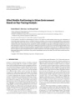
Component Separation in Wavelet Space for CMB Analysis 2441 100 which contain only isotropic features. The undecimated isotropic a trous wavelet transform has been shown to be ` 10−2 well suited to the analysis of astrophysical data where transla- 10−4 tion invariance is desirable and where the emphasis is seldom 10−6 Magnitude on data compression [23]. Further, with this choice of scal- ing function, the so-called scaling equation is satisﬁed, and 10−8 therefore fast implementations of the decomposition and re- 10−10 construction steps of the a trous transform are available [23]. ` 10−12 Given a 2D data set c0 (k, l), the a trous algorithm pro- ` duces recursively a set of detail maps wi (k, l) on a dyadic res- 10−14 olution scale and a smooth approximation cJ (k, l) [23]. We 10−16 note that the lowest resolution Jmax is obviously limited by 0.05 0.1 0.15 0.2 0.25 0.3 0 the data map size. The transform is readily inverted by Reduced frequency J Figure 1: Magnitudes averaged over spectral rings of the nearly c0 ( k , l ) = c J ( k , l ) + wi (k, l), (10) isotropic cubic spline wavelet ﬁlters ψ1 , ψ2 , . . . , ψ5 used in the sim- i=1 ulations described further down. The vertical dotted lines for ν = {0.013, 0.025, 0.045, 0.09, 0.2} delimit the ﬁve frequency bands used which is a simple addition of the smooth array with the detail with SMICA in these simulations. maps. 3.2. Spectral matching in wavelet space: wSMICA We now consider using another set of ﬁlters in place of In order to deﬁne a sensible wavelet version of SMICA, we the ideal bandpass ﬁlters used by SMICA. In dealing with ﬁrst rewrite the SMICA criterion (5) in terms of covariance nonstationary data or, as a special case, with gapped data, matrices in the initial domain, where, for instance, the gaps it is especially attractive to consider ﬁnite impulse response are best described, rather than in the Fourier domain. (FIR) ﬁlters. Indeed, provided the response of such a ﬁlter is Consider a batch of T data samples Xt=1,T where t is an short enough compared to data size T and gap widths, most appropriate index depending on the dimension of the data, of the samples in the ﬁltered signal will be unaﬀected by the and the set of Q ideal bandpass ﬁlters Fq associated with the presence of gaps. Using exclusively these samples yields esti- nonoverlapping frequency domains Fq used in SMICA. De- noting by Xq (t ) the data ﬁltered through Fq , we deﬁne sam- mated covariance matrices which are not biased by the miss- ing data, at the cost of a slight increase of variance due to ple covariance matrices discarding some data samples. In the following, we use ﬁl- ters ψ1 , ψ2 , . . . , ψJ , φJ (see Figure 1) and the wavelet a trous ` T 1 X q ( t ) X q ( t )† RT,X (q) = (11) algorithm. T t =1 Consider again a batch of T regularly spaced data samples Xt=1,T . Possible gaps in the data are simply described with a obtained by averaging in the original domain. Owing to the mask µ, that is, an array of zeroes and ones of the same size as unitary property of the discrete Fourier transform, one has the data Xt=1,T with ones corresponding to samples outside nq the gaps. Denoting by W1 , W2 , . . . , WJ and CJ the wavelet RX νq , RT,X (q) = (12) scales and the smooth approximation of X , obtained with T the a trous transform and µ1 , . . . , µJ +1 the masks for the dif- ` where nq was deﬁned as the number of Fourier modes in ferent scales determined from the original mask µ knowing spectral band Fq . These matrices are estimates of RT,X (q) = the diﬀerent ﬁlter lengths, wavelet covariances are estimated E(Xq (t )Xq (t )† ), the covariance matrix of Xq (t ). Again, ac- as follows: cording to model (3), the covariance matrices are again structured as T 1 µi (t )Wi (t )Wi (t )† , RW,X (1 ≤ i ≤ J ) = RT,X (q) = ART,S (q)A† + RT,N (q), (13) l i t =1 (15) where RT,S (q) and RT,N (q) are deﬁned similarly to RT,X (q). T 1 µJ +1 (t )CJ (t )CJ (t )† , RW,X (J + 1) = Hence, minimizing the SMICA objective function (5) is then lJ +1 t =1 equivalent to minimizing Q where li is the number of nonzero samples in µi . With source nq DKL RT,X (q), ART,S (q)A† + RT,N (q) φ (θ ) = (14) and noise covariances RW,S (i), RW,N (i) deﬁned in a similar q=1 way, the covariance model in wavelet space becomes with respect to the new set of parameters θ = (A, RT,S (q), RW,X (i) = ARW,S (i)A† + RW,N (i). RT,N (q)). (16)
2442 EURASIP Journal on Applied Signal Processing (a) (b) (c) Figure 2: Samples of simulated component maps of CMB, dust, and SZ. Our wavelet-based version of SMICA consists in minimizing in the one-dimensional case and the wSMICA criterion: 3β1 3β2 3βJ βJ +1 J +1 α1 , α2 , . . . , αJ , αJ +1 = ,..., J , J , (21) † αi DKL RW,X (i), ARW,S (i)A + RW,N (i) φ (θ ) = 4 16 4 4 (17) i=1 in the two-dimensional case. The fraction 1 − βi of discarded with respect to θ = (A, RW,S (i), RW,N (i)) for some sensible points depends on scale i (even with the a trous algorithm) ` choice of the weights αi . because the length of the wavelet ﬁlter itself depends on i. The weights in the spectral mismatch (17) should be cho- However, it is roughly scale independent, if the missing data sen to reﬂect the variability of the estimate of the correspond- are large patches of much bigger size than the length of the ing covariance matrix. Examining ﬁrst (14), we see weights wavelet ﬁlters used at any scale in the wavelet decomposition. which are proportional to nq , that is, to the number of DFT Before closing, we note that the diﬀerent wavelet ﬁlter points used in computing the sample covariance matrix, be- outputs Wi (t ) are correlated due to the overlap between fre- cause this is in fact the number of uncorrelated values of X (ν) quency responses (Figure 1). Optimal inference should take entering in the estimation of RX (νq ). It is also proportional to this correlation into account but we have chosen not to do the size of the frequency domain over which RX (νq ) is eval- so and rather to stick to a simple criterion like (17) which ig- uated. Since wSMICA uses wavelet ﬁlters with only limited nores the correlations between sample covariance matrices. overlap, we choose to use the same strategy as in SMICA No big loss is expected from this choice because the wavelet since the latter amounts to using ideal bandpass ﬁlters. In bands do not overlap very much. other words, when no data points are missing, the weights for wSMICA are taken proportional to the size of the frequency 4. NUMERICAL EXPERIMENTS domains covered at each scale. This is 4.1. Simulation of realistic maps 11 11 We have simulated observations consisting of m = 6 mix- = α1 , α2 , . . . , αJ , αJ +1 , ,..., J , J (18) 24 22 tures of n = 3 components, namely, CMB, galactic dust, and SZ emissions for which templates were obtained as described in the one-dimensional case and in [16]; see Figure 2 for typical realizations. Dust emission is the greybody emission of small dust particles in our own galaxy. The intensity of emission is 33 31 α1 , α2 , . . . , αJ , αJ +1 = , ,..., J , J (19) strongly concentrated towards the galactic plane, although 4 16 44 cirrus clouds at high galactic latitudes are present as well. The dust emission law is of the form να Bν (Tdust ) where α 1.7, in the two-dimensional case. Bν (T ) is the blackbody emission law, and Tdust 17 K is the In the case of data with gaps, we must further take into account that some wavelet coeﬃcients are discarded. Let βi typical dust temperature in the interstellar medium. The Sunyaev-Zel’dovich eﬀect (SZ) is a small distortion denote the fraction of wavelets coeﬃcients which are unaf- fected by the gaps at scale i. The number of eﬀective points is of the CMB blackbody emission law caused by inverse Comp- ton scattering of CMB photons on free electrons in hot ion- reduced by this fraction and one should use the weights ized gas, present mostly in clusters of galaxies. The energetic electron, in the interaction, gives a fraction of its energy to the scattered CMB photon, shifting its frequency to a higher β1 β2 βJ βJ +1 α1 , α2 , . . . , αJ , αJ +1 = , ,..., J , J (20) value. As a result, the SZ eﬀect causes a shift in CMB photon 24 22
Component Separation in Wavelet Space for CMB Analysis 2443 (a) (b) (c) (d) (e) (f) Figure 3: Simulated observation maps based on the templates shown in Figure 2 and the mixing matrix in Table 1 for the nominal Planck HFI noise levels. Table 1: Entries of A, the mixing matrix used in our simulations. CMB Dust SZ Channel 7.452 × 10−1 3.654 × 10−2 −8.733 × 10−1 100 GHz 5.799 × 10−1 7.021 × 10−2 −4.689 × 10−1 143 GHz 3.206 × 10−1 1.449 × 10−1 −2.093 × 10−3 217 GHz 7.435 × 10−2 3.106 × 10−1 1.294 × 10−1 353 GHz 6.009 × 10−3 5.398 × 10−1 2.613 × 10−2 545 GHz 6.115 × 10−5 7.648 × 10−1 5.268 × 10−4 857 GHz energy distribution, depleting the occupation of low energy While the relative noise standard deviations between chan- levels and populating high energy levels. The net eﬀect, to nels are set according to the nominal values of the Planck HFI, we also experiment with ﬁve global noise levels at −20, ﬁrst order, is a small additive emission, negative at frequen- −6, −3, 0, and +3 dB from nominal values. Table 2 gives the cies below 217 GHz, and positive at frequencies above. A re- view on SZ eﬀect can be found in [24]. typical energy fractions that are contributed by each of the n = 3 original sources and noise, to the total energy of each of The templates, and thus the mixtures in each simulated data set, consist of 300 × 300 pixel maps corresponding to a the m = 6 mixtures, considering Planck nominal noise vari- 12.5◦ × 12.5◦ ﬁeld located at high galactic latitude. The six ance. In fact, because SMICA and wSMICA actually work on mixtures in each set mimic observations that will eventually spectral bands, a much better indication of signal-to-noise be acquired in the six frequency channels of the Planck HFI ratio in these simulations is given by Figure 4 which shows (Figure 3). The entries of the mixing matrix A used in these how noise and source energy contributions distribute with simulations actually are estimated values of the electromag- respect to frequency in the six mixtures. netic emission laws of each component at 100, 143, 217, 353, Finally, in order to investigate the impact of gaps in the 545, and 857 GHz; see Table 1. data, and the beneﬁts of using wSMICA in place of SMICA to White Gaussian noise is added to the mixtures accord- deal with these gaps, the mask shown in Figure 5 was applied ing to model (2) in order to simulate instrumental noise. onto the mixture maps. The case where no data is missing
2444 EURASIP Journal on Applied Signal Processing Table 2: Energy fraction contributed by each source to the total energy of each mixture, for the nominal noise variance on the Planck HFI channels. CMB Dust SZ Noise Channel 9.91 × 10−1 1.18 × 10−4 7.92 × 10−3 2.53 × 10−6 100 GHz 9.97 × 10−1 7.25 × 10−4 3.79 × 10−3 5.17 × 10−7 143 GHz 9.98 × 10−1 1.01 × 10−2 2.48 × 10−7 1.34 × 10−7 217 GHz 5.55 × 10−1 4.8 × 10−1 9.78 × 10−3 7.47 × 10−8 353 GHz 2.5 × 10−3 2.75 × 10−4 3.78 × 10−9 1.0 545 GHz 1.29 × 10−7 5.56 × 10−8 1.24 × 10−10 1.0 857 GHz without any mixing, that is, we take A to be the 3 × 3 identity was also considered as a reference case. Spectral matching with wSMICA is conducted using the output of the ﬁve matrix. The following steps were repeated 1000 times. wavelet ﬁlters ψ1 , . . . , ψ5 associated to higher frequency de- (i) Randomly pick one of each component maps out of tails. For the sake of comparison, SMICA is run using ﬁve the available 200 CMB maps, 30 dust maps, and 1500 bands in Fourier space which are similar to the dyadic bands SZ maps. imposed by the wavelet transform, as shown in Figure 1. This (ii) Compute covariance matrices in the ﬁve wavelet or latter choice of frequency bands is made to ease comparison Fourier bands, both with and without masking part of between SMICA and wSMICA. the maps. (iii) Normalize each source so that its total energy over the 4.2. Experiments with noise-free mixtures ﬁve bands is equal to one. Preliminary experiments were conducted in the case of van- (iv) Estimate a separating matrix by joint diagonalization ishing instrumental noise variance. In this case, the blind of the covariance matrices. component separation problem is “equivariant,” entailing These noise-free experiments are complemented using that the quality of separation on a given mixture does not “surrogate” data in order to assess the eﬀect of any non- depend at all on the mixing matrix A but only on the par- Gaussianity or nonstationarity in the source templates. We ticular realization of the sources and on the algorithm used repeat the simulations on Gaussian stationary maps gener- for separation. More speciﬁcally, in the case of SMICA and ated with the same spectra as the CMB, dust, and SZ compo- wSMICA, separation performance depends on the spectral nents. The resulting distribution of I then only reﬂects the diversity of the components and on the ability of both objec- ability of (w)SMICA to exploit the spectral diversity of the tive functions to exploit this diversity. Hence, the noise-free components independently of the other aspects of their dis- experiments in this section are indicative of the spectral di- tribution. versity of the components, of the ability of (w)SMICA to cap- The histograms on Figure 6 are for the oﬀdiagonal term ture it, and of the robustness of the (w)SMICA with respect corresponding to the residual corruption of CMB by Gaus- to missing data. sian dust in the second set of experiments (using surrogate Note that in a noise-free model, the spectral matching data). In Tables 3 and 4, the results obtained with the syn- objective boils down to an objective of joint diagonalization thetic component maps are given as well as those obtained of the covariance matrices, as shown in [25]. Hence, spectral with the surrogate Gaussian maps, in terms of the standard matching can be implemented using an eﬃcient dedicated deviations of the oﬀdiagonal entries Ii j deﬁned by (22). algorithm [26]. When working on surrogate Gaussian maps without The estimated components are related to the true one ac- masks, using covariance matrices in Fourier space or in cording to wavelet space gives similar performances. It is also satisfac- S = I S, tory, when covariances in wavelet space are used with surro- (22) gate Gaussian maps, that each computed standard deviation where I is the product of the mixing matrix used in simula- only slightly increases when a mask is applied on the data. Indeed, as a consequence of incomplete coverage, there are tions and of the separating matrix obtained by joint diago- less samples from which to estimate the covariances. This in- nalization. It also includes any normalization needed for the crease is also observed when covariance matrices in Fourier components and their estimates to have total energy in all space are used with the surrogate Gaussian maps but it can bands equal to 1. With this normalization, the square of any be as high as ﬁvefold and it does not aﬀect all the coeﬃ- oﬀdiagonal term Ii j is directly related to the residual level of contamination by component j in the recovered compo- cients equally. Although this can again be attributed to the re- nent i. Since performance in separating noise-free mixtures duced data size, the lowered spectral diversity between com- is independent of the mixing matrix, the choice of A in the ponents, because of the correlations and smoothing induced in Fourier space by the mask, is also part of the explanation. simulations is irrelevant: it does not change the distribution of I. In practice, our noise-free experiments are conducted In fact, as shown on Figure 4, CMB and dust spatial power
Component Separation in Wavelet Space for CMB Analysis 2445 100 100 CMB 10−1 10−1 10−2 CMB 10−2 10−3 10−3 Noise 10−4 Energy Energy 10−4 Noise 10−5 10−5 10−6 SZ 10−6 10−7 Dust SZ Dust 10−7 10−8 10−9 10−8 0.05 0.1 0.15 0.2 0.25 0.3 0.05 0.1 0.15 0.2 0.25 0.3 0 0 Reduced frequency Reduced frequency (a) (b) 10−1 100 10−2 10−2 CMB 10−3 10−4 Noise CMB 10−4 Energy Energy 10−6 Noise 10−5 Dust 10−8 Dust 10−6 SZ SZ 10−10 10−7 10−12 10−8 0.05 0.1 0.15 0.2 0.25 0.3 0.05 0.1 0.15 0.2 0.25 0.3 0 0 Reduced frequency Reduced frequency (c) (d) 10−1 100 10−2 10−2 Dust 10−3 Dust 10−4 10−4 10−6 Noise 10−5 Energy Energy Noise 10−6 10−8 CMB 10−7 CMB 10−10 10−8 SZ SZ 10−12 10−9 10−10 10−14 0.05 0.1 0.15 0.2 0.25 0.3 0.05 0.1 0.15 0.2 0.25 0.3 0 0 Reduced frequency Reduced frequency (e) (f) Figure 4: Energy contributed by each source and noise in each bolometer as a function of frequency, for the nominal noise variance on the Planck HFI channels: (a) 100 GHz, (b) 143 GHz, (c) 217 GHz, (d) 353 GHz, (e) 545 GHz, and (f) 857 GHz. Note how SZ is expected to be always below nominal noise, that CMB and dust strongly dominate in diﬀerent channels, and that CMB and dust spectra, without being proportional, display the same general behavior dominated by low modes. spectra are somewhat similar, that is, show low spectral di- In the case of realistic component maps, we note ﬁrst that versity, and further smoothing can only degrade the perfor- the comparison of the performance of component separation mance of the source separation algorithm based on Fourier using wavelet-based covariance matrices with and without mask again agrees with the diﬀerent data sizes, which is not covariances.
2446 EURASIP Journal on Applied Signal Processing 4.3. Realistic experiments The results of the previous section show that, in the noise- less case, using wavelet-based covariance matrices provides a simple and eﬃcient way to cancel the bad impact that gaps actually have on the performance of estimation using Fourier-based statistics. We move on to investigate the eﬀect of additive noise on SMICA and wSMICA. Picking at random one of each component maps out of (a) (b) the available 200 CMB maps, 30 dust maps, and 1500 SZ maps, 1000 sets of six synthetic mixture maps were gener- ated as previously described, for each of the 5 noise levels chosen. Then, component separation was conducted using the spectral matching algorithms SMICA and wSMICA both with and without part of the maps being masked. A typi- cal run of SMICA or wSMICA in the setting considered here (i.e., 300 by 300 maps, 6 mixtures, 3 sources, 5 wavelet scales, no constraints on the mixing matrix) takes only a few sec- onds on a 1.25 Ghz Mac G4 when coded in IDL. The same optimization techniques are used for SMICA and wSMICA (c) (d) since the two criteria have the same form. Each run of SMICA and wSMICA on the data returns es- timates A f and Aw of the mixing matrix. These estimates are subject to the indeterminacies inherent to the instantaneous linear mixture model (2). Indeed, in the case where optimiza- tion is over all parameters θ , any simultaneous permutation of the columns of A and of the lines of S leaves the model unchanged. The same occurs when exchanging a scalar pos- sibly negative factor between any column in A and the corre- sponding line in S. Therefore, columnwise comparison of A f (e) (f) and Aw to the original mixing matrix A requires ﬁrst ﬁxing these indeterminacies. This is done “by hand” after A f and Figure 5: (a) Mask used to simulate a gap in the data. (b)–(f) Mod- Aw have been normalized columnwise. iﬁed masks at scales 1 through 5. The discarded pixels are in black. The results we report next focus on the statistical proper- ties of A f and Aw as estimated from the 1000 runs of the two competing methods in the several conﬁgurations retained. In the case with covariances in Fourier space. Next, whether fact, the correct estimation of the mixing matrix in model covariance matrices are computed in Fourier space or in (2) is a relevant issue, for instance, when it comes to deal- wavelet space, we note that the terms coupling CMB and ing with the cross-calibration of the diﬀerent detectors. Fig- dust are again much higher than with surrogate data, even ures 7, 8, and 9 show the results obtained, using the quadratic on complete maps. This is probably to be attributed to the norm nonstationarity and/or non-Gaussianity of the Dust com- ponent. Another point is that the CMB and dust templates 1/ 2 m 2 as in Figure 2 exhibit sharp edges compared to SZ and this QE j = Ai j − Ai j (23) inevitably disturbs spectral estimation using a simple DFT. i =1 To assess this eﬀect, simulations were also conducted where the covariances in Fourier space were computed after an with A = A f or Aw and j = CMB, dust, or SZ, to assess the apodizing Hanning window was applied on the complete residual errors on the estimated emissivities of each compo- data maps. The results reported in Table 3, to be compared nent. The plotted curves show how the mean of the above to Table 4, do indicate a slightly positive eﬀect of windowing, positive error measure varies with increasing noise variance. but still the separation using wavelet-based statistics appears For the particular case of CMB, Table 6 gives the estimated better. To further complete this preliminary study, we con- standard deviations of the relative errors (Ai j −Ai j )/Ai j on the ducted similar experiments using JADE [27], an ICA algo- estimated CMB emission law in the six channels of Planck’s rithm based on fourth-order statistics. This algorithm does HFI in the diﬀerent conﬁgurations retained. not use spectral information at all. As discussed earlier, such Closer to our source separation objective, a more signif- a method is not expected to work well on CMB data and the results reported in Table 5 do show lower performance icant way of assessing the quality of A f and Aw as estima- in comparison to Tables 3 and 4. tors of the mixing matrix A would be to use the following
Component Separation in Wavelet Space for CMB Analysis 2447 0.25 0.25 0.2 0.2 Proportion of counts Proportion of counts 0.15 0.15 0.1 0.1 0.05 0.05 0 0 −0.1 −0.05 −0.1 −0.05 0.05 0.1 0.05 0.1 0 0 Oﬀdiagonal entry Oﬀdiagonal entry (a) (b) Figure 6: Histograms of the oﬀdiagonal term of I, deﬁned in (22), corresponding to the residual corruption of “CMB” by “dust” while separating Gaussian maps generated with the same power spectra as the astrophysical components, by joint diagonalization of covariance matrices in (a) Fourier and (b) wavelet spaces, with (black, which appears grey when seen through white ) and without (white) masking part of the data. The dark widest histogram on the left highlights the impact of masking on source separation based on Fourier covariance matrices. Table 3: Standard deviations of the oﬀdiagonal entries Ii j deﬁned by (22) obtained while separating realistic component maps by joint diagonalization of covariance matrices in Fourier space, with (M ) or without masking (NM ) part of the data, or applying an apodizing Hanning window (Han). Components 1, 2, and 3, respectively, stand for CMB, dust, and SZ. The numbers in italic were obtained with Gaussian maps and the underlined numbers correspond to the histograms in Figure 6. Oﬀdiag. entry NM M Han I1,2 0.097 0.074 0.024 0.0076 0.038 I1,3 0.0049 0.005 0.0094 0.0044 0.006 I2,1 0.017 0.018 0.017 0.0066 0.01 I2,3 0.0064 0.0066 0.011 0.0077 0.0096 I3,1 0.0024 0.0028 0.0039 0.0026 0.0037 I3,2 0.0054 0.0054 0.01 0.0071 0.0079 Table 4: Standard deviations of the oﬀdiagonal entries Ii j deﬁned by (22) obtained while separating realistic component maps by joint diagonalization of covariance matrices in wavelet space, with (M ) and without masking (NM ) part of the data. Components 1, 2, and 3, respectively, stand for CMB, dust, and SZ. The numbers in italic were obtained with Gaussian maps and the underlined numbers correspond to the histograms in Figure 6. Oﬀdiag. entry NM M I1,2 0.015 0.018 0.0071 0.0079 I1,3 0.0025 0.0028 0.0029 0.0031 I2,1 0.016 0.019 0.0077 0.0089 I2,3 0.0041 0.0048 0.0051 0.0075 I3,1 0.0024 0.003 0.0029 0.0039 I3,2 0.0039 0.0053 0.0054 0.0085
2448 EURASIP Journal on Applied Signal Processing Table 5: Standard deviations of the oﬀdiagonal entries Ii j deﬁned Regarding future work, a few points are in order. First, by (22) obtained while separating realistic component maps using we note that possible correlations between the components JADE, with (M ) and without masking (NM ) part of the data. Com- are not accounted for in SMICA or wSMICA as presented ponents 1, 2, and 3, respectively, stand for CMB, dust, and SZ. here. However, it is not diﬃcult in principle to handle such known or suspected correlations by adding oﬀdiagonal pa- Oﬀdiag. entry I1,2 I1,3 I2,1 I2,3 I3,1 I3,2 rameters in the model spectral covariances of the sources. NM 0.021 0.25 0.022 0.02 0.31 0.02 Still, in the case of CMB analysis from high frequency obser- M 0.023 0.29 0.025 0.018 0.34 0.018 vations which contain only one galactic component (dust) as in our simulations, spatial correlations between components should not be a problem. interference-to-signal ratio: We note that the proposed wavelet-based approach, as implemented with the standard a trous wavelet transform, ` i= j I j ,i σi 22 oﬀers little ﬂexibility in the spectral bands available for wS- ISR j = , (24) I j, j σ 2 2 MICA while the Fourier approach gives complete ﬂexibility j in this respect. But it is possible, even straightforward, to use where the σ j are the source variances and other transforms such as the a trous wavelet packet trans- ` form, or the continuous wavelet transform, or in fact any set −1 I = A† R−1 A A† R−1 A of linear ﬁlters, preferably FIR ﬁlters. This in turn raises the (25) N N question of optimally choosing this set of ﬁlters, keeping in mind that higher resolution in Fourier space requires longer with RN the noise covariance. The plots on Figures 10, 11, ﬁlters, which is not desirable in the case of incomplete or and 12 show how the mean ISR from the 1000 runs of SMICA and wSMICA in diﬀerent conﬁgurations varies with increas- nonstationary data. In fact, the optimal selection of bands is clearly a meaningful question both for SMICA and wSMICA. ing noise. Figure 13 typically estimated component maps ob- We also note that in the CMB application, the com- tained using SMICA and wSMICA. For the sake of compari- ponents have quite diﬀerent statistical properties: some are son, component maps estimated using the JADE source sep- expected to be very close to Gaussian (like the CMB) aration method are also included. whereas others are strongly non-Gaussian (like SZ). The We note again that the performance of wSMICA behaves non-Gaussianity of some components does not aﬀect the as expected when noise increases and if part of the data is consistency of our estimator but, for a given spectrum, it missing. However, this is not always the case with SMICA. does aﬀect the distribution of the estimates although this im- Finally, this set of simulations, conducted in a more realistic pact is not easily predicted. It is clear, however, that ignoring setting with respect to ESA’s Planck mission, again conﬁrms the strong non-Gaussianity of some components is a loss of the higher performance, over Fourier analysis, that we indeed information. Devising a method able, with reasonable com- expected from the use of wavelets. The latter are able to cor- plexity, to exploit jointly non-Gaussianity (as in traditional rectly grab the spectral content of partly masked data maps ICA techniques) and spectral information (as in Fourier or and from there allow for better component separation. wavelet SMICA) appears as a diﬃcult challenge. 5. CONCLUSION APPENDIX This paper has presented an extension of the spectral match- ing ICA algorithm to the wavelet domain, motivated by EM ALGORITHM WITH CONSTRAINTS ON the need to deal with components which exhibit spatial THE MIXING MATRIX correlations and are nonstationary. Maps with gaps are a Considering Q separate frequency bands of size nq with particular instance of practical signiﬁcance. Substituting co- nq = 1, the EM functional derived for the instanta- variance matching in Fourier space by covariance matching neous mixing model (2) with independent Gaussian station- in wavelet space makes it possible to cope with gaps of any ary sources S and noise N is shape in a very straightforward manner. Mainly, it is the ﬁnite length of the wavelet ﬁlters used here that allows the impact Φ(θ , θ ) = E log p X , S|θ |θ (A.1) of edges and gaps on the estimated covariances and hence on component separation to be lowered. Optimally choosing the with θ = (A, RS,1 , . . . , RS,Q , RN ,1 , . . . , RN ,Q ) and θ = (A, FIR ﬁlter bank regarding a particular application is a possible RS,1 , . . . , RS,Q , RN ,1 , . . . , RN ,Q ). The maximization step of the further enhancement. EM algorithm seeks then to maximize Φ(θ , θ ) with respect Our numerical experiments, based on realistic simula- to θ and the optimal θ is used as the value for θ at the next tions of the astrophysical data expected from the Planck mis- EM step, and so on until satisfactory convergence is reached. sion, conﬁrm the beneﬁts of correctly processing existing Explicit expressions are easily derived for the optimal θ in the gaps. Clearly, other possible types of nonstationarities in the white noise case where an interesting decoupling occurs be- collected data such as spatially varying noise or component tween the reestimating equations for noise variances, source variance, and so forth could be dealt with very simply in a variances, and the mixing matrix [15]. similar fashion using the wavelet extension of SMICA.
Component Separation in Wavelet Space for CMB Analysis 2449 0.008 Mean squared error Mean squared error 0.006 10−1 0.005 0.004 10−2 0.003 −20 −6 −3 −20 −6 −3 0 3 0 3 Noise level in dB relative to nominal values Noise level in dB relative to nominal values Fourier + Hanning Wavelet + no mask Fourier + Hanning Wavelet + no mask Fourier + mask Wavelet + mask Fourier + mask Wavelet + mask Fourier + no mask Fourier + no mask Figure 7: Comparison of the mean squared errors on the estima- Figure 9: Comparison of the mean squared errors on the estima- tion of the emission law of SZ as a function of noise in ﬁve diﬀerent tion of the emission law of CMB as a function of noise in ﬁve dif- ferent conﬁgurations: wSMICA without mask, wSMICA with mask, conﬁgurations: wSMICA without mask, wSMICA with mask, fS- fSMICA without mask, and fSMICA with mask, and fSMICA with MICA without mask, fSMICA with mask, and fSMICA with Han- Hanning apodizing window. ning apodizing window. 0.4 First, we exhibit the quadratic dependence of the EM functional Φ(θ , θ ) on A: 0.3 Φ( θ , θ ) Mean squared error 0.2 1 nq trace ARss A† R−1q − ARxs† R−1q − Rxs A† R−1q =− q N, q N, q N, 2q + constA , (A.2) 0.1 where −1 Cq = A† R−1q A + R−,1 , 0.05 N, Sq −20 −6 −3 0 3 −1 Wq = A† R−1q A + R−,1 A† R−1q , Noise level in dB relative to nominal values N, Sq N, (A.3) † Rxs = RX ,q Wq , Fourier + Hanning Wavelet + no mask q Fourier + mask Wavelet + mask † Rss = Wq RX ,q Wq + Cq . Fourier + no mask q Figure 8: Comparison of the mean squared errors on the estima- In the white noise case, RN ,q = RN , (A.2) becomes tion of the emission law of dust as a function of noise in ﬁve diﬀer- ent conﬁgurations: wSMICA without mask, wSMICA with mask, 1 † A − Rxs Rss−1 Rss A − Rxs Rss−1 R−1 Φ(θ , θ ) = − trace fSMICA without mask, and fSMICA with mask, and fSMICA with N 2 Hanning apodizing window. + constA , (A.4) Linear equality constraints where When A is subject to linear constraints, the joint maximiza- tion of the EM functional with respect to all model parame- Rxs = nq Rxs , Rss = nq Rss . (A.5) ters is no longer easily achieved in general. In fact, one cannot q q q q simply decouple the reestimating rules for the noise param- eters and the mixing matrix and these have to be optimized Again, this can be rewritten as separately. We give next the modiﬁed reestimating equations 1 for the mixing matrix and the source variances in the case of Φ(θ , θ ) = − (A − M)† Q(A − M) + constA , (A.6) constant noise (i.e., θ = (A, RS,1 , . . . , RS,Q )). 2
2450 EURASIP Journal on Applied Signal Processing Table 6: Standard deviations of the relative errors on the estimated emission laws Ai1 of CMB in Planck’s HFI six channels. The column labels WNM, WM, FNM, FM, FHan are for the diﬀerent conﬁgurations, respectively: wSMICA without mask, wSMICA with mask, fSMICA without mask, fSMICA with mask, and fSMICA with Hanning apodizing window. The ﬁve ﬁgures in each box are for noise variance -20, -6, -3, 0, and 3 dB from nominal Planck values. Emission law WNM WM FNM FM FHan 4.4 ∗ 10−4 5.0 ∗ 10−4 6.2 ∗ 10−4 7.3 ∗ 10−4 7.2 ∗ 10−4 5.4 ∗ 10−4 7.5 ∗ 10−4 7.1 ∗ 10−4 8.5 ∗ 10−4 9.5 ∗ 10−4 A11 6.6 ∗ 10−4 9.2 ∗ 10−4 8.2 ∗ 10−4 8.9 ∗ 10−4 1.3 ∗ 10−3 −4 −3 −3 −3 1.7 ∗ 10−3 9.4 ∗ 10 1.2 ∗ 10 1.0 ∗ 10 1.0 ∗ 10 1.2 ∗ 10−3 1.7 ∗ 10−3 1.2 ∗ 10−3 1.4 ∗ 10−3 2.3 ∗ 10−3 1.6 ∗ 10−4 2.1 ∗ 10−4 2.1 ∗ 10−4 2.0 ∗ 10−4 2.7 ∗ 10−4 5.3 ∗ 10−4 7.8 ∗ 10−4 5.6 ∗ 10−4 5.7 ∗ 10−4 1.0 ∗ 10−3 A21 −4 −3 −4 −4 1.4 ∗ 10−3 7.0 ∗ 10 1.1 ∗ 10 7.6 ∗ 10 8.4 ∗ 10 1.0 ∗ 10−3 1.6 ∗ 10−3 1.0 ∗ 10−3 1.0 ∗ 10−3 2.1 ∗ 10−3 −3 −3 −3 −3 3.1 ∗ 10−3 1.4 ∗ 10 2.2 ∗ 10 1.5 ∗ 10 1.7 ∗ 10 1.5 ∗ 10−3 1.8 ∗ 10−3 2.2 ∗ 10−3 2.5 ∗ 10−3 2.3 ∗ 10−3 1.7 ∗ 10−3 2.1 ∗ 10−3 2.3 ∗ 10−3 2.6 ∗ 10−3 2.9 ∗ 10−3 A31 2.1 ∗ 10−3 2.6 ∗ 10−3 2.6 ∗ 10−3 2.8 ∗ 10−3 3.7 ∗ 10−3 −3 −3 −3 −3 4.2 ∗ 10−3 2.7 ∗ 10 3.0 ∗ 10 2.9 ∗ 10 3.0 ∗ 10 3.3 ∗ 10−3 4.6 ∗ 10−3 3.3 ∗ 10−3 3.5 ∗ 10−3 6.1 ∗ 10−3 1.8 ∗ 10−2 2.0 ∗ 10−2 2.7 ∗ 10−2 3.0 ∗ 10−2 2.5 ∗ 10−2 −2 −2 −2 −2 2.7 ∗ 10−2 1.9 ∗ 10 2.1 ∗ 10 2.7 ∗ 10 2.1 ∗ 10 A41 2.1 ∗ 10−2 2.4 ∗ 10−2 2.8 ∗ 10−2 3.1 ∗ 10−2 2.9 ∗ 10−2 2.7 ∗ 10−2 2.8 ∗ 10−2 3.1 ∗ 10−2 3.0 ∗ 10−2 3.5 ∗ 10−2 −2 −2 −2 −2 4.9 ∗ 10−2 3.0 ∗ 10 4.1 ∗ 10 2.5 ∗ 10 2.7 ∗ 10 4.0 ∗ 10−1 4.5 ∗ 10−1 6.1 ∗ 10−1 6.6 ∗ 10−1 5.6 ∗ 10−1 4.2 ∗ 10−1 4.7 ∗ 10−1 6.1 ∗ 10−1 6.5 ∗ 10−1 5.8 ∗ 10−1 A51 −1 −1 −1 −1 6.4 ∗ 10−1 4.5 ∗ 10 5.0 ∗ 10 6.1 ∗ 10 6.7 ∗ 10 5.7 ∗ 10−1 5.9 ∗ 10−1 6.7 ∗ 10−1 6.7 ∗ 10−1 7.5 ∗ 10−1 6.2 ∗ 10−1 8.4 ∗ 10−1 5.0 ∗ 10−1 5.5 ∗ 10−1 1.0 5.7 ∗ 101 6.2 ∗ 101 8.5 ∗ 101 9.2 ∗ 101 7.8 ∗ 101 5.8 ∗ 101 6.5 ∗ 101 8.6 ∗ 101 9.1 ∗ 101 8.1 ∗ 101 A61 6.2 ∗ 101 6.9 ∗ 101 8.6 ∗ 101 9.4 ∗ 101 8.9 ∗ 101 ∗ 101 ∗ 101 ∗ 101 9.2 ∗ 101 1.0 ∗ 102 7.9 8.2 9.3 8.6 ∗ 101 1.2 ∗ 102 6.9 ∗ 101 7.7 ∗ 101 1.4 ∗ 102 where C is a matrix with as many columns as constraints, and where the columns of C have the same size as A. The maximum of Q = RN −1 ⊗ A = vect A, nq Rss , the EM functional with respect to θ subject to the speciﬁed q q linear constraints is then reached for  −1   (A.7) −1   A = M − Q−1 C C † Q−1 C C † M − A0 , M = vect  nq Rxs   nq Rss   . q q (A.9) q q RS,q = diag Rss , q Here “vect” builds a column vector with the entries of a ma- trix taken along its rows. Now we consider linear constraints where “diag” returns a diagonal matrix with the same diago- on the mixing matrix, speciﬁed as follows: nal entries as its input argument. In the free noise case, things are quite similar except that C † A − A0 = 0, (A.8) the noise covariance matrices RN ,q do not factor out as nicely.
Component Separation in Wavelet Space for CMB Analysis 2451 10−2 10−2 Mean interference-to-signal ratio Mean interference-to-signal ratio 10−3 10−3 10−4 10−4 10−5 10−5 −20 −6 −3 −20 −6 −3 0 3 0 3 Noise level in dB relative to nominal values Noise level in dB relative to nominal values Wavelet + no mask Fourier + no mask Wavelet + no mask Fourier + no mask Fourier + mask Wavelet + mask Wavelet + mask Fourier + mask Fourier + Hanning Fourier + Hanning Figure 12: Comparison of the mean ISR for SZ as a function of Figure 10: Comparison of the mean ISR for CMB as a function noise in ﬁve diﬀerent conﬁgurations, namely, wSMICA without of noise in ﬁve diﬀerent conﬁgurations, namely, wSMICA without mask, wSMICA with mask, fSMICA without mask, fSMICA with mask, wSMICA with mask, fSMICA without mask, and fSMICA mask, and fSMICA with Hanning apodizing window. with mask, and fSMICA with Hanning apodizing window. 10−2 Then, the maximum of the EM functional with respect to θ subject to the speciﬁed linear constraints is again reached for Mean interference-to-signal ratio −1 A = M − Q−1 C C † Q−1 C C † M − A0 , (A.12) 10−3 RS,q = diag Rss . q These expressions of the reestimates of the mixing matrix can become algorithmically very simple when, for instance, the linear constraints to be dealt with aﬀect separate lines of A, 10−4 or even simpler when the constraints are such that the entries −20 −6 −3 0 3 of A are aﬀected separately. Noise level in dB relative to nominal values Wavelet + no mask Fourier + no mask Positivity constraints on the entries of A Wavelet + mask Fourier + mask Fourier + Hanning Suppose a subset of entries of A are constrained to be posi- tive. The maximization step of the EM algorithm on A alone, Figure 11: Comparison of the mean ISR for dust as a function of noise in ﬁve diﬀerent conﬁgurations, namely, wSMICA without again has to be modiﬁed. We suggest dealing with such con- straints in a combinatorial way rephrasing the problem in mask, wSMICA with mask, fSMICA without mask, fSMICA with mask, and fSMICA with Hanning apodizing window. terms of equality constraints. If the unconstrained maximum of the EM functional is not in the speciﬁed domain, then one has to look for a maximum on the borders of that do- The EM functional is again expressed as main: on a hyperplane, on the intersection of two, three, or more hyperplanes. One important point is that the maxi- 1 mum of the EM functional with respect to A subject to a Φ(θ , θ ) = − (A − M)† Q(A − M) + constA , (A.10) 2 set of equality constraints will necessarily be lower than the maximum of the same functional considering any subset of where in this case these equality constraints. Hence, not all combinations need be explored, and a branch-and-bound-type algorithm is well nq R−1q ⊗ Rss , nq R−1q Rxs . suited [28]. A straightforward extension allows to deal with M = Q−1 vect Q= N, N, q q the case where a set of entries of the mixing matrix is con- q q (A.11) strained by upper and lower bounds.
2452 EURASIP Journal on Applied Signal Processing (a) (b) (c) (d) (e) (f) (g) (h) (i) (j) (k) (l) Figure 13: (a)–(f) Estimated component maps obtained with SMICA and wSMICA, respectively. These estimates result from applying a Wiener ﬁlter in each frequency band or wavelet scale based on the optimized model parameters (see Section 2.3). (g)–(i) The initial source templates after applying the optimal Wiener ﬁlter obtained with SMICA, that is, the same as (a)–(c) but leaving out noise and residual contaminations. (j)–(l) Maps estimated using JADE [27]. The initial source maps are shown in Figure 2. REFERENCES [2] A. Benoˆt, P. Ade, A. Amblard, et al., “Archeops: a high ı resolution, large sky coverage balloon experiment for map- [1] G. F. Smoot, C. L. Bennett, A. Kogut, et al., “Structure in the ping cosmic microwave background anisotropies,” Astropar- COBE diﬀerential microwave radiometer ﬁrst-year maps,” As- ticle Physics, vol. 17, no. 2, pp. 101–124, 2002. trophysical Journal Letters, vol. 396, no. 1, pp. L1–L5, 1992. [3] P. de Bernardis, P. Ade, J. J. Bock, et al., “A ﬂat universe from
Component Separation in Wavelet Space for CMB Analysis 2453 high-resolution maps of the cosmic microwave background [19] M. M. Ichir and A. Mohammad-Djafari, “Wavelet domain radiation,” Nature, vol. 404, no. 6781, pp. 955–959, 2000. blind image separation,” in Wavelets: Applications in Signal [4] S. Hanany, P. Ade, A. Balbi, et al., “MAXIMA-1: a measure- and Image Processing X, vol. 5207 of Proceedings of SPIE, pp. ment of the cosmic microwave background anisotropy on an- 361–370, San Diego, Calif, USA, November 2003. gular scales of 10 arcminutes to 5 degrees,” Astrophysical Jour- [20] G. Patanchon, J. Delabrouille, and J.-F. Cardoso, “Source sep- nal Letters, vol. 545, pp. L5–L9, 2000. aration on astrophysical data sets from the WMAP satellite,” [5] C. L. Bennett, M. Halpern, G. Hinshaw, et al., “First year in Proc. 5th International Conference on Independent Com- Wilkinson microwave anisotropy probe (WMAP) observa- ponent Analysis (ICA ’04), pp. 1221–1228, Granada, Spain, tions: preliminary maps and basic results,” Astrophysical Jour- September 2004. nal Supplement Series, vol. 148, no. 1, pp. 1–27, 2003. [21] J.-F. Cardoso and D.-T. Pham, “Optimization issues in noisy [6] G. Jungman, M. Kamionkowski, A. Kosowsky, and D. N. Gaussian ICA,” in Proc. 5th International Conference on Inde- Spergel, “Cosmological-parameter determination with mi- pendent Component Analysis (ICA ’04), pp. 41–48, Granada, crowave background maps,” Physical Review D, vol. 54, no. 2, Spain, September 2004. ´ pp. 1332–1344, 1996. [22] E. Hivon, K. M. Gorski, C. B. Netterﬁeld, B. P. Crill, S. Prunet, [7] F. R. Bouchet and R. Gispert, “Foregrounds and CMB exper- and F. Hansen, “MASTER of the cosmic microwave back- iments: I. Semi-analytical estimates of contamination,” New ground anisotropy power spectrum: A fast method for sta- Astronomy, vol. 4, no. 6, pp. 443–479, 1999. tistical analysis of large and complex cosmic microwave back- [8] M. Tegmark and G. Efstathiou, “A method for subtracting ground data sets,” The Astrophysical Journal, vol. 567, no. 1, foregrounds from multi-frequency CMB sky maps,” Monthly pp. 2–17, 2002. Notices of the Royal Astronomical Society, vol. 281, no. 4, [23] J.-L. Starck, F. Murtagh, and A. Bijaoui, Image and Data Anal- pp. 1297–1314, 1996. ysis: The Multiscale Approach, Cambridge University Press, [9] M. P. Hobson, A. W. Jones, A. N. Lasenby, and F. R. Bouchet, Cambridge, UK, 1998. [24] M. Birkinshaw, “The Sunyaev-Zel’dovich eﬀect,” Physics Re- “Foreground separation methods for satellite observations of the cosmic microwave background,” Monthly Notices of the ports, vol. 310, no. 2-3, pp. 97–195, 1999. Royal Astronomical Society, vol. 300, no. 1, pp. 1–29, 1998. [25] D.-T. Pham, “Blind separation of instantaneous mixture of [10] M. Tegmark, D. J. Eisenstein, W. Hu, and A. de Oliveira-Costa, sources via the Gaussian mutual information criterion,” Sig- “Foregrounds and forecasts for the cosmic microwave back- nal Processing, vol. 81, no. 4, pp. 855–870, 2001. ground,” The Astrophysical Journal, vol. 530, no. 1, pp. 133– [26] D. T. Pham, “Joint approximate diagonalization of posi- 165, 2000. tive deﬁnite hermitian matrices,” SIAM Journal on Matrix [11] C. Baccigalupi, L. Bedini, C. Burigana, et al., “Neural net- Analysis and Applications, vol. 22, no. 4, pp. 1136–1152, works and the separation of cosmic microwave background 2001. and astrophysical signals in sky maps,” Monthly Notices of the [27] J.-F. Cardoso, “High-order constrasts for independent com- Royal Astronomical Society, vol. 318, no. 3, pp. 769–780, 2000. ponent analysis,” Neural Computation, vol. 11, no. 1, pp. 157– [12] D. Maino, A. Farusi, C. Baccigalupi, et al., “All-sky astrophys- 192, 1999. ical component separation with fast independent component [28] P. Narendra and K. Fukunaga, “A branch and bound al- analysis (FASTICA),” Monthly Notices of the Royal Astronomi- gorithm for feature subset selection,” IEEE Trans. Comput., cal Society, vol. 334, no. 1, pp. 53–68, 2002. vol. 26, no. 9, pp. 917–922, 1977. [13] E. E. Kuruoglu, L. Bedini, M. T. Paratore, E. Salerno, and A. Tonazzini, “Source separation in astrophysical maps using in- Y. Moudden graduated in electrical en- dependent factor analysis,” Neural Networks, vol. 16, no. 3-4, gineering from SUPELEC, Gif-sur-Yvette, pp. 479–491, 2003. France, and obtained an M.S. degree in [14] H. Snoussi, G. Patanchon, J. Macias-Perez, A. Mohammad- Djafari, and J. Delabrouille, “Bayesian blind component sep- ´ physics from the Universite de Paris VII, aration for cosmic microwave background observations,” in France, in 1997. He received a Ph.D. degree Bayesian Inference and Maximum Entropy Methods, MaxEnt ´ in signal processing from the Universite de Workshops, pp. 125–140, American Institute of Physics, New Paris XI, Orsay, France. He was a Visitor at York, NY, USA, August 2001. UCLA in 2004 and is currently a Postdoco- [15] J.-F. Cardoso, H. Snoussi, J. Delabrouille, and G. Patanchon, toral Fellow with the CEA, Saclay, France, “Blind separation of noisy Gaussian stationary sources. Ap- working on applications of signal process- plication to cosmic microwave background imaging,” in Proc. ing to astronomy. His research interests include signal and image 11th European Signal Processing Conference (EUSIPCO ’02), processing, data analysis, and statistics and information theory. vol. 1, pp. 561–564, Toulouse, France, September 2002. [16] J. Delabrouille, J.-F. Cardoso, and G. Patanchon, “Multidetec- J.-F. Cardoso is with the French “Cen- tor multicomponent spectral matching and applications for tre National de la Recherche Scientiﬁque” cosmic microwave background data analysis,” Monthly Notices (CNRS), in the Signal and Image Processing of the Royal Astronomical Society, vol. 346, no. 4, pp. 1089– ´ ´ Department, Ecole Nationale Superieure 1102, 2003. ´´ des Telecommunications (ENST, Paris). His [17] J.-F. Cardoso, “The three easy routes to independent com- research area is statistical signal processing. ponent analysis; contrasts and geometry,” in Proc. 3rd Inter- Since 1989, he has been extensively working national Conference on Independent Component Analysis (ICA on all aspects of blind source separation and ’01), San Diego, Calif, USA, December 2001. independent component analysis. In 2001, [18] M. Zibulevsky and B. A. Pearlmutter, “Blind source separa- he started a collaboration with astronomers tion by sparse decomposition in a signal dictionary,” Neural and cosmologists for the statistical analysis of astronomic data. Computation, vol. 13, no. 4, pp. 863–882, 2001.
2454 EURASIP Journal on Applied Signal Processing J.-L. Starck has a Ph.D. degree from Uni- versity Nice-Sophia Antipolis and a Habil- itation from University Paris XI. He was a Visitor at the European Southern Observa- tory (ESO) in 1993, at UCLA in 2004, and at Stanford’s Statistics Department in 2000 and 2005. He has been a researcher at CEA since 1994. His research interests include image processing and statistical methods in astrophysics and cosmology. He is also the author of two books entitled Image Processing and Data Analysis: The Multiscale Approach (Cambridge University Press, 1998), and Astronomical Image and Data Analysis (Springer, 2002). J. Delabrouille graduated in 1991 from the ´ ´ ´´ “Ecole Nationale Superieure des Telecom- munications” with a major in aerospace telecommunication (1991). He then ob- tained in 1998 a Ph.D. degree in physics from the University of Chicago and a Ph.D. degree in astrophysics and space techniques from the University of Orsay. He is cur- rently employed by CNRS in the Astropar- ticle and Cosmology (APC) Laboratory in Paris, where he is the Head of the Data Analysis and Simulation Group. His main research interests are in cosmology and gravita- tion, cosmic microwave background observations, and developing methods for complex data analysis.