


Báo cáo hóa học: " Generic Hardware Architectures for Sampling and Resampling in Particle Filters"
lượt xem 4
download
 Download
Vui lòng tải xuống để xem tài liệu đầy đủ
Download
Vui lòng tải xuống để xem tài liệu đầy đủ
Tuyển tập báo cáo các nghiên cứu khoa học quốc tế ngành hóa học dành cho các bạn yêu hóa học tham khảo đề tài: Generic Hardware Architectures for Sampling and Resampling in Particle Filters
Bình luận(0) Đăng nhập để gửi bình luận!
Nội dung Text: Báo cáo hóa học: " Generic Hardware Architectures for Sampling and Resampling in Particle Filters"
- EURASIP Journal on Applied Signal Processing 2005:17, 2888–2902 c 2005 Hindawi Publishing Corporation Generic Hardware Architectures for Sampling and Resampling in Particle Filters Akshay Athalye Department of Electrical and Computer Engineering, Stony Brook University, Stony Brook, NY 11794-2350, USA Email: athalye@ece.sunysb.edu ´ Miodrag Bolic Department of Electrical and Computer Engineering, Stony Brook University, Stony Brook, NY 11794-2350, USA Email: mbolic@ece.sunysb.edu Sangjin Hong Department of Electrical and Computer Engineering, Stony Brook University, Stony Brook, NY 11794-2350, USA Email: snjhong@ece.sunysb.edu ´ Petar M. Djuric Department of Electrical and Computer Engineering, Stony Brook University, Stony Brook, NY 11794-2350, USA Email: djuric@ece.sunysb.edu Received 18 June 2004; Revised 11 April 2005; Recommended for Publication by Markus Rupp Particle filtering is a statistical signal processing methodology that has recently gained popularity in solving several problems in signal processing and communications. Particle filters (PFs) have been shown to outperform traditional filters in important prac- tical scenarios. However their computational complexity and lack of dedicated hardware for real-time processing have adversely affected their use in real-time applications. In this paper, we present generic architectures for the implementation of the most com- monly used PF, namely, the sampling importance resampling filter (SIRF). These provide a generic framework for the hardware realization of the SIRF applied to any model. The proposed architectures significantly reduce the memory requirement of the filter in hardware as compared to a straightforward implementation based on the traditional algorithm. We propose two architectures each based on a different resampling mechanism. Further, modifications of these architectures for acceleration of resampling pro- cess are presented. We evaluate these schemes based on resource usage and latency. The platform used for the evaluations is the Xilinx Virtex II pro FPGA. The architectures presented here have led to the development of the first hardware (FPGA) prototype for the particle filter applied to the bearings-only tracking problem. Keywords and phrases: particle filters, hardware architectures, memory schemes, real-time processing, bearings-only tracking. 1. INTRODUCTION PFs are Bayesian in nature and their goal is to find an approximation to the posterior density of a state of interest (e.g., position of a moving object in tracking, or transmit- Particle filters (PFs) [1, 2] are used to perform filtering for ted symbol in communications) based on corrupted obser- models that are described using the dynamic state-space ap- vations which are inputs to the filter. In the traditional PFs proach [1]. Many problems in signal processing and commu- known as sample importance resample filters (SIRFs), this nications can be described using these models [3]. In most posterior is represented by a random measure consisting of a practical scenarios, these models are nonlinear, the states weighted set of samples (particles). The particles are drawn are high-dimensional, and the densities involved are non- or sampled from a density known as the importance function Gaussian. Traditional filters like the extended Kalman fil- (IF) using the principle of importance sampling (IS) [1]. This ter (EKF) are known to perform poorly in such scenarios [4]. PFs on the other hand are not affected by the condi- sampling step is followed by the importance computation step which assigns weights to the drawn particles based on tions of nonlinearity and non-Gaussianity and handle high- received observations using IS rules to form the weighted set dimensional states better than traditional filters [5].
- Hardware Architectures for Sampling and Resampling in PFs 2889 of particles. Another important process called resampling is scheme 2, respectively. As we will see later, the resampling generally needed in PFs to avoid weight degeneracy [2]. Var- operation in the SIRFs presents a bottleneck since it is in- ious estimates of the state like MMSE or MAP estimates can herently sequential and also cannot be executed concurrently be calculated from this weighted set of particles. The number (pipelined) with other operations. Scheme 1 has a low com- of particles used to compute the posterior depends upon the plexity and simple control structure, but is generically slow nature of application, dimension of the state, and the per- since SR involves a while loop inside an outer for loop. As formance requirements. From here on, we will refer to the opposed to this, the RSR algorithm has a single for loop number of particles used as M and the dimension of the state and hence scheme 2 is faster than scheme 1. We also pro- as Ns . pose modifications of these schemes which bring about par- tial parallelization of resampling and reduce the effect of the The main drawback of SIRFs is their computational com- plexity. For each observation received, all the M particles resampling bottleneck on execution throughput. need to be processed through the steps of sampling, impor- The rest of the paper is organized as follows. In Section 2 tance computation, and resampling. The sampling and im- we briefly describe the theory behind the SIRF, the tradi- portance computation steps typically involve transcenden- tional SR algorithm, and the new RSR algorithm. Section 3 tal exponential and nonlinear operations. Once all the M presents the proposed architectures and their modification particles have been processed through the above-mentioned for increased speed. Evaluation of resource utilization and steps, the estimate of the state at the sampling instant is cal- latency of the two schemes on FPGA platform along with an culated and the next input can be processed. These opera- example application is presented in Section 4. Section 5 con- tions present significant computational load even on a state- cludes the paper. of-the-art DSP. The performance of SIRF for the bearings- only tracking problem [6] with Ns = 4 was evaluated on TI 2. BACKGROUND TMS320C54x generation DSP [7]. With M = 1000 particles, the inputs to the filter could be processed at the rate of only 2.1. The SIRF algorithm 1 kHz. Clearly this speed would prevent the use of PFs for on- Dynamic state space (DSS) models to which SIRFs can be line signal processing in real-time applications where higher applied are of the form sampling rates and/or higher number of particles are needed for processing. Thus, design of dedicated hardware for SIRF xn = fn xn−1 , qn , (1) is needed if real-time applications are to become feasible. SIRF is a recursive algorithm. The sampling step uses the yn = gn xn , vn , (2) resampled particles of the previous instant to compute the particles of the current instant. This requires the particles where fn and gn are possibly nonlinear functions describ- to be stored in memories. We will see later that a straight- ing the DSS model. The symbol xn represents the dynami- forward implementation of the traditional SIRF algorithm cally evolving state of the system, qn represents the process would have a memory requirement of 2Ns × M since sam- noise, and yn is the observation vector of the system which pled and resampled particles need to be stored in differ- is corrupted by the measurement noise vn at instant n. The ent memories. Most practical applications involve nonlin- SIRF algorithm estimates the state of the system xn based on ear models and high-dimensional states (large Ns ) which im- the received corrupted observations. The algorithm proceeds plies a large number of particles M for SIRFs applied to these through the following steps. problems [8]. This would make the total memory require- (1) Sampling step (S). In this step, samples (particles) of ment of 2Ns × M very large. The architectures proposed in the unknown state are drawn from the IF. In our implemen- this paper reduce this memory requirement to Ns memories tation we choose the prior probability density function (pdf) of depth M (i.e., Ns × M ). This not only reduces the hard- of the state, given by p(xn | xn−1 ) to be the IF. This prior pdf ware resource requirement of the SIRF but also makes it more can be deduced from (1). The sampling step can be thought energy-efficient due to reduced memory accesses [9]. of as propagation of particles at time instant n − 1 into time The specifics of an SIRF implementation depend upon instant n through (1). The sampled set of particles at instant the properties of the model to which the SIRF is applied. n is denoted by {xnm) }M=0 . The SIRF is initialized with a prior ( −1 m However, from a hardware viewpoint, the high-level data set of particles at time instant 0 to start the recursion. These flow and control structure remain the same for every model. particles are then successively propagated in time. This paper focuses on the development of efficient architec- (2) Importance (weight) computation step (I). This step tures for these generic operations of the SIRF. They include assigns importance weights wnm) to the particles xnm) based ( ( the resampling step and memory-related operations of the on the received observations. This step is the most compu- sample step. The other model-dependent operations are data tationally intensive and generally involves the computation driven and involve mathematical computations. They can be of transcendental trigonometric and exponential functions. easily incorporated into the proposed architectures for any Since we use the prior IF for our implementation, the weight model. We develop two architectures, one using the tradi- assignment equation is tional systematic resampling (SR) algorithm and the other using the new residual systematic resampling (RSR) algo- wnm) = wnm) · p yn | xnm) . ( ( ( (3) rithm. These architectures are referred to as scheme 1 and −1
- 2890 EURASIP Journal on Applied Signal Processing resampling algorithm for PFs [1]. This algorithm functions for m = 0 to M − 1 by resampling with replacement from the original set of par- (1) Sampling step. Draw sample xnm) from p(xn | xnm) ). ( ( −1 ticles {xnm) }M=0 to obtain a new set {xnm) }M=0 , where resam- ( ( −1 −1 (2) Importance computation step. Calculate the weight m m wnm) = p( yn | xnm) ). ( ( pling is carried out according to end ( j) ( j) Pr xni) = xn ( = wn . (4) (3) Resampling step. Determine the resampled set of particles {xnm) }M=0 ( −1 m (4) Output calculation. Calculate the desired (like In other words, the particles drawn in the sample step MMSE, MAP) estimate of the state xn . and their weights form a distribution. The Resampled parti- cles are drawn proportional to this distribution to replace the Pseudocode 1: SIRF algorithm. original set. The normalized weights of all resampled parti- cles are set to 1/M . The SR concept for a PF that used 5 particles is shown Input observations yn in Figure 2a. First the cumulative sum of weights (CSW) of sampled particles is computed. This is presented in the figure for the case of 5 particles (M = 5) with weights w(0) , . . . , w(4) . Then, as shown on the y axis of the graph, a function u(m) xn wn xn , wn Importance called the resampling function is systematically updated [1] Sampling Resampling computation and compared with the CSW of the particles. The corre- Output sponding particles are replicated to form the resampled set estimate which for this case is {x(0) , x(0) , x(3) , x(3) , x(3) }. In the tradi- tional SR algorithm, it is essential for the weights to be nor- Figure 1: Overall structure of the SIRF. malized such that their sum is one. However we use a mod- ified resampling algorithm that avoids weight normalization by incorporating the sum of weights into the resampling The implementation of this step is largely dependent on the operation [10]. This avoids M divisions per SIRF recursion nature of the DSS model for the particular problem at hand which is very advantageous for hardware implementation. and therefore is not discussed in this paper. The determination of the resampled set of particles is (3) Resampling step (R). Resampling prevents degener- done sequentially as is shown in Figure 2b. In each cycle, de- ation of particle weights by eliminating particles with small pending on the results of comparison between the two num- weights and replicating particles with large weights to replace bers U and CSW, which represent the current value of the those eliminated. This replication or discarding is done based resampling function and the CSW respectively, the relevant on some function of the particle weights. The resampled set particle is replicated or discarded and the value of either the of particles is denoted by {xnm) }M=0 , and the weights of these ( −1 resampling function U or the cumulative sum of weights m particles after resampling are denoted by {wnm) }M=0 , which ( −1 CSW is updated. As shown in the figure, in the first cycle, m are typically 1/M . The resampled particles along with their u(0) and csw(0) are compared. Since CSW > U , particle 0 is weights form a random measure {xnm) , wnm) }M=0 which is ( ( −1 replicated and the resampling function is updated, while in m used to represent the posterior p(xn | y1:n ) and calculate es- cycle 4, since CSW < U , particle 1 is discarded and the CSW timates of the state. is updated. This process is repeated till the replicated set of The SIRF algorithm is summarized in Pseudocode 1. particles is obtained. As we will see later, the SR algorithm needs 2M − 1 cycles Figure 1 shows the overall structure of the SIRF. The recur- sive nature of the filter can be seen from the presented data for execution in hardware. flow. The sample and importance steps can be pipelined in 2.3. Residual systematic resampling algorithm operation. Resampling requires knowledge of sum of all par- ticle weights. Hence it cannot begin before the weights of In spite of the low hardware complexity, the low speed of all the particles have been calculated. The sample step of the SR algorithm may not be tolerable in case of high-speed time n + 1 cannot begin until resample step of time n has applications. For these cases, the residual systematic resam- been completed. Thus, resampling cannot be executed con- pling (RSR) algorithm proposed in [11] can be used. This currently with any other operation and presents a bottleneck algorithm has a single for loop of M iterations and hence is which limits the sampling rate of the SIRF. The architectures twice faster than SR in terms of number of cycles. This al- presented in this paper reduce the effect of this bottleneck gorithm is based on the traditional residual resampling algo- by using efficient memory schemes and modified resampling rithm [12]. In residual resampling (RR) the number of repli- algorithms. cations of a specific particle x(m) is determined by truncating the product of the number of particles M and the particle 2.2. Systematic resampling in SIRF weight w(m) . The result is known as a replication factor. The The first architecture proposed in this paper uses the system- sum of the replication factors of all particles, except for some atic resampling algorithm. This is the most commonly used special cases, is less than M . These remaining particles are
- Hardware Architectures for Sampling and Resampling in PFs 2891 CSW csw(4) 3 u(4) csw(3) 3 Resampled set u(3) 3 csw(2) u(2) csw(1) 0 u(1) csw(0) 0 u(0) 0 1 2 3 4 m (a) CSW(0) CSW Cycle 1 u(0) Replicate particle 0 U CSW(0) CSW Cycle 2 u(0) u(1) U Update U , replicate particle 0 CSW(0) CSW Cycle 3 u(0) u(1) u(2) Update U , no result U CSW(1) CSW(0) CSW Cycle 4 u(0) u(1) u(2) Update CSW, discard particle 1 U (1) (2) CSW CSW CSW(0) CSW Cycle 5 u(0) u(1) u(2) Update CSW, discard particle 2 U ··· (b) Figure 2: The concept of systematic resampling. (a) Resampling using cdfs. (b) Resampling done sequentially. latency of the RSR datapath LRSR is typically low (LRSR = 2 obtained from the residues of the truncated products using for our implementation). The RSR algorithm for M particles some other mechanisms like systematic resampling or ran- dom resampling. RR thus requires two loops of M iterations: is summarized in Pseudocode 2. one for processing the truncated products and the other for Figure 3 graphically illustrates the RSR methods for the case of M = 5 particles. The RSR algorithm draws the processing residues. RSR calculates the replication factor of uniform random number U (0) = ∆U (0) and updates it by each particle similar to RR but it avoids the second loop of ∆U (m) = ∆U (m−1) + r (m) /M − wnm) . The difference ∆U (m) be- ( RR by including the processing of the residues by systematic resampling in the same loop. This is done by combining the tween the updated uniform number and the current weight is propagated. Figure 3 shows that r (0) = 2, that is, particle 0 resampling function U with the truncated product. As a re- is replicated twice, r (3) = 3, that is, particle 3 is replicated 3 sult, this algorithm has only one loop and the processing time is independent of the distribution of the weights at the input. times, and all other particles are discarded. SR and RSR pro- The RSR has an execution time of M + LRSR cycles, where the duce identical resampling result.
- 2892 EURASIP Journal on Applied Signal Processing −1 determines the resampled set of particles {xn }M=0 , which are m (r ) = RSR(M , w) written to the memory labelled RMEM. The sample unit 1 (1) Generate a random number ∆U (0) ∼ U 0, then reads particles from RMEM for propagation. These M memories are shown in Figure 4a for Ns = 1. (2) for m = 0 to M − 1 r (m) = (wnm) − ∆U (m−1) ) · M + 1 ( The memory schemes proposed here reduce this require- (3) r (m) ment to Ns memories of depth M . In our implementation, (m) ∆U (m) = ∆U (m−1) + − wn (4) M the resampling unit returns the set of indexes (pointers) of (5) end the replicated particles instead of the particles themselves. Then indirect addressing [13] can be used to read the set −1 Pseudocode 2: Residual systematic resampling (RSR) algorithm. {xn }M=0 from the sample memory SMEM itself for propa- m gation. This means that the particles are propagated in the following manner: xnm) ∼ p xn | xn−1m) , ind( ( (6) ∆U (4) W (4) where ind(m) represents the array of indexes or pointers to the resampled particles. Here we make use of the fact that W (3) the resampled particles are in fact a subset of the particles in the sampled particles memory. Hence instead of replicat- ing them and storing them in a different memory, they can ∆U (3) be read from the same memory by using appropriate point- ∆U (2) ∆U (1) W (2) ers. The sampling process involves reading of M resampled W (1) particles and writing of M sampled particles to the memory. If a single port memory is used the reads and writes cannot be done simultaneously. This would require that a resampled W (0) particle be read, propagated, and written to the memory be- ∆U (0) fore the next resampled particle can be read. The execution of the sample step would then take 2(M + LS ) cycles where LS 0 1 2 3 4 is the latency of sample computation. Particle This execution can be speeded up by using dual-port Figure 3: Residual systematic resampling for an example with M = memories [14] which are readily available on an FPGA plat- −1 form.1 This enables reading of {xn−1 }M=0 and writing of 5 particles. m (m) M −1 {xn }m=0 to be executed concurrently. Hence, the sample step for M particles can be done in M + LS cycles. The mem- 3. ARCHITECTURES AND MEMORY SCHEMES ory scheme is shown in Figure 4b where the single dual-port memory labelled PMEM replaces the memories SMEM and We now elaborate on the development of architectures for RMEM of Figure 4a. Thus, use of index addressing reduces the SIRF employing each of the two resampling mechanisms the memory requirement of the SIRF and use of dual-port discussed in the previous section. memories reduces the execution cycle time. However, using index addressing alone does not ensure 3.1. Reduction of memory requirement that the scheme with the single memory will work correctly. In the SIRF algorithm, the sampled particles {xnm) }M=0 are ( −1 m We illustrate the reason for this with a simple example. generated by propagating the previous resampled particles Consider the following one-dimensional random walk ( m) −1 {xn−1 }M=0 . This is done in the following manner using the model: m DSS model: xn = xn−1 + qn , (7) xnm) ∼ p xn | xnm) , ( ( m = 0, 1, . . . , M − 1. yn = xn + vn . (5) −1 Here xn represents the one-dimensional state of the A straightforward implementation of the SIRF would system and yn is a noisy measurement. The symbols qn require 2 × Ns memories of depth M , Ns for storing the and vn are the process and the measurement noises, re- sampled particles {xnm) }M=0 , and Ns for storing the resam- ( −1 spectively. Consider 5 sampled particles at instant n − 1 m (m) M −1 pled particles {xn }m=0 . This implementation is shown in (i.e., {xnm) }4 =0 ). In the implementation of Figure 4a, these ( −1 m Figure 4a. At time instant n, the sampled particles {xnm) }M=0 ( −1 m will be stored in the memory labelled SMEM. Their weights will be calculated in the importance computation step. Once 1 We would like to point out here that on an ASIC platform, use of dual- all the weights have been determined, the resampling unit port memories incurs a 2x area penalty.
- Hardware Architectures for Sampling and Resampling in PFs 2893 Write/read successively Write/read from 0 to M − 1 Resampled successively particles from 0 to M − 1 of instant ‘n − 1’ Resampled Sampled Sampled Sample Importance Resample particles particles particles (RMEM) of instant ‘n’ (SMEM) (a) Resampled Use pointers particles to replicated particles of instant ‘n − 1’ Address Read Sample Importance Resample port Use relevant PMEM addresses Address Write port Sampled particles Data of instant ‘n’ (b) Figure 4: Memories for storing particles. In the traditional implementation two memories would be needed. These are replaced by a single dual-port memory. (a) Resampling requiring two memories. (b) Modified architecture needing only one dual-port memory. (0) (0) (0) (0) SMEM[0] = xn = RMEM[0] + qn = PMEM[0] + qn xn (1) (1) (1) (1) SMEM[1] = xn = RMEM[1] + qn = PMEM[0] + qn xn (2) (2) (2) (2) SMEM[2] = xn = RMEM[2] + qn = PMEM[3] + qn xn (3) (3) (3) (3) SMEM[3] = xn = RMEM[3] + qn = PMEM[3] + qn xn (4) (4) (4) (4) SMEM[4] = xn = RMEM[4] + qn = PMEM[3] + qn xn (a) (b) Figure 5: Memory operations in sample step, (a) for implementation with two memories and (b)for implementation with one memory. particles will be stored in the memory SMEM at loca- indexes. For this example, the set of indexes of replicated par- ticles is {0, 0, 3, 3, 3}. Thus the operations of the sample step tions SMEM[0], . . . , SMEM[4]. Suppose that after resam- (0) (3) will be as shown in Figure 5b. However, if sampled particles pling, particle xn−1 is replicated twice, xn−1 three times, and are written to successive locations of PMEM as in the previ- (1) (2) (4) that particles xn−1 , xn−1 , and xn−1 are discarded. In the imple- ous case, the particle xnm) will overwrite the resampled par- ( mentation with two memories, the resampled particles will (m) ticle xn−1 causing an error if this particle has been replicated be written to memory RMEM. The operations performed (0) in the sample step at instant n for this case are shown in multiple times. In the above example, if the particle xn is Figure 5a. written to PMEM[0], then for the next particle, we will get As seen from the figure, the sampled particles are written (1) (0) (1) xn = xn + qn (8) to the memory SMEM. In the reduced memory implementa- which is incorrect. Thus different strategies for writing sam- tion of Figure 4b, the replicated particles are read out of the same single memory (PMEM in this case) using resampled pled particles to the memory need to be devised for the
- 2894 EURASIP Journal on Applied Signal Processing Out C2 enable Counter2 (C2) To C2 enable Address C1 Particle Replicated enable Counter1 index W particle Particle U ≤W CSW MEM (C1) index index (MEM1) Particle memory index Write en (MEM2) Index Subtractor generator (compare) Particle index Discarded particle Write en index U FIFO Accum. Accum. U >W Reg enable To C1 To accum. u0 enable enable Figure 6: Architecture of resampling unit implementing SR. Rep Read index Address Reg Rep Read port PREG Sample unit PMEM Read index (latency LS ) Address Discarded index Write port Data Figure 7: Architecture of sample unit. reduced memory design to function correctly. In the follow- (propagated) particles back to the memory. A particle, which ing sections, we will explain the architectures developed us- has been generated by a replication, is written to the loca- ing SR and RSR and how they handle reading and writing of tion of a discarded particle in the memory. The number of the particle memory. particles before and after resampling is the same. This means that for every replicated particle there will be a discarded par- ticle. Hence this scheme can be used effectively for writing 3.2. SIRF using systematic resampling: scheme 1 particles to the memory. Since the number of particles that Figure 6 shows the architecture for the resampling unit im- will be discarded is nondeterministic, we use a FIFO buffer plementing the SR mechanism. The CSW is stored in the of depth M to store the discarded particle indexes. The out- memory labelled MEM1 at locations corresponding to the put of counter C1 at an instant is the index of the particle that ordinal number of the particle in the sampled set. The re- sampling function u(m) is generated using an accumulator as is currently being processed. The comparator and the index generator unit bring about the resampling as in Figure 2. If shown. Both the memory and the accumulator are controlled the particle is replicated, its index is written to MEM2 whose by enable signals. The outputs of the accumulator and the memory (U and W ) are compared for conditions U ≤ W locations are addressed by counter C2, and the accumulator is enabled so as to update the value of the resampling func- and U > W by using a subtractor. The values of the CSW tion. If the particle is discarded or when all its replications are read from the memory using one counter (C1). The re- are found, counter C1 is enabled CSW of the next particle sults of the comparison are passed to the index generator unit is read from the memory. When an index is to be discarded, which determines whether to replicate or discard the particle the write enable of the FIFO buffer is asserted and the index (i.e., the index of the particle). The indexes of the replicated is written to it. particles are stored in the memory MEM2. Figure 7 shows the architecture for the sample step under This scheme also records the indexes of the discarded this scheme. Once resampling is done, the memory MEM2 particles. These indexes are used while writing the sampled
- Hardware Architectures for Sampling and Resampling in PFs 2895 0 1 0 2 3 4 3 3 Replicated Discarded indexes FIFO indexes (MEM2) (a) (b) Figure 8: Addressing read and write ports of particle memory using stored indexes. (a) Contents of memory and FIFO after resampling. (b) Reading of replicated and discarded indexes. Table 1: Function of sample step. Note that writing of particles is done LS cycles after they are read, where LS is the latency of the sample unit. Cycle Read address Replication Read from Write to 1 0 No PMEM[0] PMEM[0] 2 0 Yes PREG PMEM[1] 3 3 No PMEM[3] PMEM[3] 4 3 Yes PREG PMEM[2] 5 3 Yes PREG PMEM[4] represents the array ind(m) containing M replicated indexes. We now further illustrate this scheme with our previous ex- This memory is read sequentially and the indexes are used as ample. addresses to the read port of the dual-port memory (PMEM) Following the same case of the example, the contents of storing the particles. The output of this memory is the set the replicated index memory MEM2 and discarded index −1 {xn }M=0 . Due to the nature of the SR algorithm, all the repli- FIFO in Figure 6 will be as shown in Figure 8a. The sample m cations of a particular index will be written to successive lo- step starts by reading of the content of MEM2. The opera- cations in MEM2. Thus, since this memory is read sequen- tions in various cycles are listed in Table 1. Figure 8b shows tially, a replication can be detected by comparing the cur- how the FIFO is read. A replication is detected by compar- rent read index with the previous one. When an index is read ing the current read index with the previous one. From the from MEM2 for the first time, the corresponding particle is index memory contents, we see that in this case a replication read from the memory and stored in the temporary register will be indicated when MEM2[1], MEM2[3], and MEM2[4] PREG. After propagation this particle is written to its original are read. The result of this comparison is used as read enable location in the memory. When the same index is read from to the FIFO. SR involves comparison of M values of the CSW with MEM2 in the following cycle, replication is detected, and the M values of the resampling function. As seen in Figure 2b, particle is read from the temporary register PREG rather than from the memory (since the location in the memory will be the two functions cannot be updated simultaneously, except overwritten by the propagated particle). Also, the read enable when obtaining their initial values at the start of resampling. of the FIFO is asserted high and a discarded index is obtained The result of the comparison in each cycle indicates which which is used as address to the write port of PMEM to write function is to be updated. Thus execution of SR requires 2M − 1 cycles. the replicated particle after propagation (see Figure 8b).
- 2896 EURASIP Journal on Applied Signal Processing 3.3. Modification of scheme 1 for Replicated 0 2 indexes reduced execution time 3 3 Some properties of the SR algorithm can be used to partially 4 0 parallelize resampling at the cost of added hardware. Due to the systematic nature of the resampling func- 2 0 Discarded tion update, the final value of the resampling function is 1 0 indexes fixed. This value is u(0) + (M − 1)/M for traditional SR and Replicated and Replication u(0) + S(M − 1)/M for our implementation of resampling us- discarded indexes factors ing nonnormalized weights [10]. Also the final value of the CSW, S, is also known to us. We can use this property of SR to Figure 9: Contents of memories after the RSR method with particle split the resampling shown in Figure 2a into two concurrent allocation with arranged indexes. loops of M/ 2 iterations each. One loop determines the first M/ 2 resampled indexes by comparing csw(0) to csw(M/2−1) (i, r ) = RSR(M , S, w) with u(0) to u(M/2−1) and the other loop determines the next (1) Generate a random number U ∼ U[0, 1] M/ 2 resampled indexes by comparing csw(M/2) to csw(M −1) (2) K = M/S with u(M/2) to u(M −1) . From a hardware viewpoint, this would (3) indr = 0, indd = M − 1 (4) for m = 1 to M require reading of two values of the CSW simultaneously temp = wnm) · K − U // Temporary variable ( (5) from the memory which can be accomplished by storing fact = temp (6) the CSW values (MEM1 in Figure 6) in a dual-port mem- U = fact − temp (7) ory. Also the replicated particle index memory MEM2 would if fact > 0 // Particle allocation (8) need to be dual port and the discarded index FIFO would be i(indr ) = m, r (indr ) = fact, indr = indr +1 (9) replaced by two FIFOs of half the size. All other logic blocks (10) else i(indd ) = m, r (indd ) = 0, indd = indd −1 (11) in Figure 6 would be replicated. This would reduce the loop (12) end bound [15] of the SIRF recursion and increase its through- (13) end put. With this scheme, SR is split up into two parallel loops of M/ 2 iterations each. Execution time of SR is reduced to Pseudocode 3: Modified residual systematic resampling (RSR) al- 2 × M/ 2 − 1 = M − 1 cycles at the cost of added hardware. As gorithm. an extension of this concept, resampling can be split up into more than 2 loops of simultaneous comparisons due to the systematic update of the resampling function. However this From an implementation viewpoint, the RSR algorithm would need more memory blocks and additional hardware. is beneficial since it has a single for loop. To make the RSR al- The tradeoff between added hardware and obtained speed is gorithm suitable for implementation, we make some changes considered in Section 4. in Pseudocode 2 in Section 2.3. The changes incorporate par- ticle allocation with arranged indexes in the algorithm and 3.4. SIRF with residual systematic also allow for resampling using nonnormalized weights. As in resampling: scheme 2 the case of SR, this saves M divisions at each instant. The second architecture introduced in this paper uses the The modified RSR algorithm is shown in Pseudocode 3. RSR mechanism for resampling. The RSR has only one loop In Pseudocode 3, there is one multiplication inside the of M iterations and is faster than the SR. In this scheme too, loop and one division before the loop. The incorporation of the number K and generation of U from U[0, 1] is done to the replicated particles are written to the locations of the dis- carded particles in the same dual-port particle memory. Un- allow nonnormalized weights in the resampling algorithm. These changes do not affect the correctness of the algo- like scheme 1, after resampling in this scheme the indexes of all the particles are stored in one index memory. Another rithm and the resampling results produced are the same as memory is used to store the corresponding replication factors. Pseudocode 2. If an index has been discarded, a factor of 0 is recorded at the Lines 9 and 11 bring about particle allocation with ar- corresponding location in the replication factors memory. In ranged indexes by writing replicated and discarded indexes this scheme, the indexes are arranged in such a way that all to the top and bottom parts of the index memory, respec- replicated indexes are written to the memory starting from tively. location 0 up, while all discarded indexes are written to loca- The memory-related operations in the sample step are tions from M − 1 down. This method of storing indexes and shown in Pseudocode 4. First, the replicated indexes are read replication factors is called particle allocation with arranged sequentially from the memory of arranged indexes as shown indexes. in the first for loop (line 2). The corresponding replication Memory usage for the example described in Section 3.1 factors of the indexes are also read at the same time. If the is shown in Figure 9, where the indexes are arranged in the particle has been replicated, then it is propagated repeatedly. memory using the above-mentioned method and the corre- This is shown by the second for loop (line 5) whose iterations sponding replication factors are stored in a separate mem- equal the replication factor for that particular index. Then, r (indr ) − 1 sampled particles are written to the addresses of ory.
- Hardware Architectures for Sampling and Resampling in PFs 2897 (X ) = Sampling (i, r , X ) concurrent loops. The modified algorithm for 2 concurrent (1) indr = 0, indd = M − 1 loops is shown in Pseudocode 5. The first loop does the usual (2) for indr = 1 to length(indr ) RSR of Pseudocode 3 for the first M/ 2 particles from index 0 Reg = X (i(indr )) (3) to M/ 2 − 1. The second loop does the same simultaneously X (i(indr )) = Sample (Reg), indr = indr +1 (4) for the remaining particles from index M/ 2 to M . This algo- for k = r (indr ) − 1 down to 1 (5) rithm needs the cumulative sum of weights of the first M/ 2 X (i(indd )) = Sample (Reg), indd = indd −1 (6) particles. This is denoted as SM/2 . The initial value of the re- (7) end sampling function for the second loop is denoted by U 2 in (8) end the pseudocode. Once again the factor K is included so as to allow resampling using nonnormalized weights. This mecha- Pseudocode 4: Memory-related operations of the sample step. nism can also be directly extended to include more than two loops at the cost of adding more memory and hardware. the discarded particles (line 6) by reading the arranged index The execution time is thus reduced to (M/ 2)+2+ L1 cycles memory from the bottom. The first sampled particle rewrites where the additional latency L1 is introduced by the compu- the original replicated particle (line 3). Hence the replicated tation of r M/2−1 and U 2 before the second loop can start. particle has to be stored in a variable Reg. 3.5. Architecture for scheme 2 4. EVALUATION In this section, the architectures for the algorithms presented In this section, we present the results of the implementation in Pseudocodes 3 and 4 are shown in Figures 10 and 11. In and a comparison of the two proposed architectures. Both Figure 10, weights are stored in the memory MEMw and ad- architectures were captured using Verilog HDL and synthe- dressed by the address counter that counts from 0 to M − 1 sized on a Xilinx Virtex 2 pro FPGA platform. The design and corresponds to the variable m in Pseudocode 3. The in- was verified using Modelsim from Mentor Graphics. After dex generator is the block in which the arithmetics from verification, the Verilog description was used as input to the the lines 5, 6, and 7 from Pseudocode 3 are implemented. Xilinx Development System which synthesized, mapped, and The other part of the figure represents the implementation placed and routed the designs on a Xilinx Virtex 2 pro de- of the particle allocation step (lines 8–12 of Pseudocode 3). vice (XC2VP50-ff1152). The implemented design was veri- MEMi stores the arranged indexes and MEMr stores the cor- fied through a post place and route simulation using Model- responding replication factors. Depending on whether a par- sim. ticle is replicated or not, its index is written to MEMi at ad- dress pointed to by either the counter counting up (counterr ) 4.1. Execution time or the counter counting down (counterd ). The appropriate replication factor is written to the corresponding location in Figure 12 shows the timing of operations for one recursion MEMr . of the SIRF. In the figure, LS and LI represent the startup la- There are three main blocks in Figure 11: address gener- tencies of the sample and importance unit, respectively. Tres ation, address control, and particle generation and storing. is the number of cycles required for resampling. The total cy- cle time of the SIRF is then TSIRF = (M + LS + LI + Tres )Tclk , One dual-port memory PMEM is used for storing particles. The arithmetics of the sampling step is implemented in the where Tclk is the system clock period. sampling unit. The delay between read and write operations As can be seen from the timing diagram, the resampling for the memory PMEM is determined by the pipeline latency step is a bottleneck in the SIRF execution as it cannot be of the sample unit (LS ). It is presented as Delay1 in the fig- pipelined with other operations. Thus, Tres significantly af- ure. Counter f represents the variable k in Pseudocode 4. The fects the cycle time TSIRF . Hence, developement of faster and more efficient resampling algorithms is vital to the imple- replication from the memory MEMr is used as the initial value to the down counter counter f . The other logic blocks mentation of real-time particle filters in high-speed appli- are for generation of controls to bring about sampling as de- cations. The architectures and their modifications that have scribed in Pseudocode 4. been presented in this paper help to bring down Tres in dif- ferent ways and hence reduce the effect of the resampling 3.6. Modification of scheme 2 for bottleneck. A resampling scheme should be chosen such that reduced execution time its time Tres satisfies the required TSIRF for the application at hand. The modified versions of the two resampling schemes The RSR algorithm needs M +LRSR cycles for execution where partially parallelize resampling and reduce execution time at the latency due to pipelining of the RSR datapath is LRSR (2 the cost of added hardware. The times Tres and TSIRF needed in our case). Similar to the SR, the RSR algorithm can also be for resampling and one SIRF recursion respectively in terms parallelized with addition of more hardware for reduced ex- of cycles are summarized in Table 2. k is the number of loops ecution time. The RSR algorithm used for scheme 2 has only into which resampling is split as described in Sections 3.3 and one loop in which the replication factor of a particle is deter- 3.6 for modified schemes. mined and the value of the resampling function is systemati- In the table, L accounts for the startup latencies of all the cally updated. This algorithm can also be modified for paral- units in the respective schemes. lel execution by splitting the resampling process into multiple
- 2898 EURASIP Journal on Applied Signal Processing Resampling Particle allocation En Counter d Indd Address Replicated down Replication Particle =0 and Wight index (m) factors (r ) W discarded Index Counter W memory Comp. generator index up En Counter r Indr (MEMW ) >0 memory up Data (MEMi) En Write en Delay1 Address Replicated factors memory Data (MEMr ) Figure 10: The architecture for the RSR algorithm combined with the particle propagation. Address generation Particle generation and storing Indr Replicated En Counter r up and Address discarded id , ir Sample index X En Reg memory Address Counter d unit (Latency LS ) down (MEMi) Indd Select Delay1 Read port Write en En Address Replicated PMEM r factor Control logic memory Address (MEMr ) Write port Data Address control Figure 11: The architecture for memory-related operations of the sampling step. Samplen Samplen+1 Importancen Importancen+1 Resamplen LS M + LI Tres TSIRF Figure 12: Timing of operations in SIRF. 4.2. Resource utilization the chip. The memory required by SIRF for processing a cer- tain number of particles depends upon the dimension of the The architectures presented in the paper include all the state and the number of bits used in the fixed point repre- memory-related operations of the generic SIRF. We use a Vir- sentation of the state, weights (or CSW), and indexes. The tex 2 pro FPGA platform for evaluation [16]. All memory number of 18 kb blocks needed on the Virtex 2 pro device modules are mapped to the 18 kb block RAMs available on
- Hardware Architectures for Sampling and Resampling in PFs 2899 Table 2: Timing of SIRF using the different proposed architectures. Modified scheme 1 Modified scheme 2 Time (cycles) Scheme 1 Scheme 2 with k loops with k loops M M 2M − 1 −1 Tres M + Lrsr + LRSR 2 k 2 k+2 k+1 TSIRF 3M + L 2M + L M+L M+L k k Table 3: Resource utilization for the two schemes on the XC2VP50-ff1152 device. Scheme 1 Scheme 2 Modified scheme 1 Modified scheme 2 Resource (implemented) (implemented) (estimated) (estimated) k · 199 k · 294 Slices 199 294 k · 130 k · 224 Slice registers 130 224 k · 232 k · 348 4 input LUTs 232 348 k k Block RAMS 15 14 11 + 10 + 2 2 k Block multipliers 0 1 0 Table 4: Comparison of memory requirement and cycle time with a straightforward implementation. Straightforward Parameter Scheme 1 Scheme 2 implementation 2 · Ns · M Ns · M + 2 Ns · M + 2 Memory (words) 4 · M + L(SR) 3·M+L 2·M+L TSIRF (cycles) 3 · M + L(RSR) and are represented using log2 M = 11-bits. The indexes and for storing M particles (also weights, CSWs, or indexes), BM , is given by weights are obviously one-dimensional and the particles for the BOT problem are 4-dimensional. Accordingly, the num- M·b ber of memory blocks needed for each of these can be cal- BM = Ns , (9) 18 × 1024 culated from (9). The total memory requirement of the two schemes for the mentioned bit widths is shown in Table 3. Scheme 1 requires more memory than scheme 2 since it where b is the number of bits used for representation of the needs to store the CSW which has a wider fixed point rep- word in the memory. resentation. The amount of block RAMs available on a par- Table 3 summarizes the total utilization of the proposed ticular FPGA will determine the number of particles that an architectures. The model we have chosen for our evaluation is the Ns = 4 dimensional bearings-only tracking (BOT) SIRF realization on that device can process. Thus, (9) can be used as a guideline for selecting a device for a particular im- problem [6]. The fixed point widths in the design of this pro- plementation. The mathematical units in scheme 2 like the totype were chosen using a methodology similar to that in adders and multiplier were chosen to be 18-bits wide in input [17]. Here a statistical analysis of all the variables in the al- and output. The table also gives an estimate of the resources gorithm over several runs is performed. The first 4 moments needed for the modified implementations of the two schemes of the value that a particular variable takes are used to de- with resampling being split into k parallel loops. termine a fixed point format for representing that variable Finally, Table 4 shows the comparison of cycle time in hardware within a tolerable error of 10% to 15% for dif- and memory requirement (in terms of words) for the pro- ferent variables. This analysis will need to be done for ev- posed schemes with a straightforward implementation start- ery model before the SIRF is applied to it. The chosen bit widths will not only affect the memory utilization as in (9), ing from the traditional algorithm. This approach requires the sampled and resampled particles to be stored in different but will also increase latencies LS and LI . However, these la- memories. Also if the index-addressing schemes presented tencies are small as compared to M and hence TSIRF will not be significantly affected by bit widths. For the BOT model, here are not used, another M cycles are added to the SIRF we have used an 18-bit representation for the M = 2048 execution time since resampled particles first need to be read from one memory and written to another before the sample particles and the weights and 25-bit representation for the step can begin. CSW. The indexes and replication factors are whole numbers
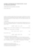
- 2900 EURASIP Journal on Applied Signal Processing Table 5: Resource utilization for entire SIRF for the bearings-only tracking problem using scheme 1. Random no. Importance Top level Sample Resample Resource Total generation computation logic Slices 300 411 1535 199 623 3068 (13%) Slice registers 364 568 2578 130 752 4392 (10%) 4 input LUTs 196 404 2674 232 342 3848 (8%) Block RAMs 2 8 1 7 0 18 (8%) Block multipliers 6 0 3 0 4 13 (6%) 0 SIRF for the BOT problem. Random number generation is needed for the sample step in accordance with the state space −1 model. We have used a quantized version of the Box-Muller method for generating the random numbers. The impor- −2 tance step in the model involves exponential and arctangent operations and hence has a high resource requirement. These −3 y position are implemented using 2 pipelined CORDIC units. The re- −4 sults of the tracking are shown in Figure 13. The position es- timates are obtained from a post place and route simulation −5 of the SIRF. The outputs are 32-bits wide and are in fixed point format. Their values are interpreted using SystemC −6 fixed point data types and plotted using MATLAB. The figure −7 also shows the tracking results obtained by the SIRF run in MATLAB using floating point representation for all variables. −8 These results are also compared with tracking results ob- −0.25 −0.2 −0.15 −0.1 −0.05 0 tained with the traditional EKF which for this model has ex- x position ecution speed of 10 kHz on a DSP platform (TMS320C54x). True state SIRF in hardware This performance figure of 16 kHz is for 2048 particles. SIRF in MATLAB EKF In practice a much larger number of particles is needed for Figure 13: Results of tracking for the BOT problem. tracking in noisy environments. This makes the SIRF compu- tationally very intensive, and real-time processing using any software platform or DSP is not possible even for low sample 4.3. Example application rates. The FPGA hardware SIRF on the other hand can pro- The entire SIRF along with the computational units of sam- cess input samples at rates of upto 3.5 kHz even with 10 000 pling and importance for the above-mentioned bearings- particles using the basic scheme 1. Large number of parti- only tracking problem was implemented on a Xilinx Vir- cles will lead to increased memory requirement. But a large tex II pro device (XC2VP50FF1152). This FPGA prototype FPGA like the one chosen for our evaluation will support a used the architecture described in scheme 1 with a resam- high number of particles. Thus, the hardware realization of pling time Tres = 2M − 1 cycles as explained earlier. The state the SIRF not only allows for increased sample rates but also in this model is 4-dimensional and incorporates the position enables real-time processing even with a very large number coordinates and velocities in x and y directions, respectively. of particles. The input to the filter is the time varying angle (bearing) of By using the other schemes introduced in the paper, the the moving object with respect to a fixed measurement point. SIRF can be made even faster. Currently, work is being done This input is sampled by the filter at rate 1/TSIRF . Each input on the development of parallel architectures for the SIRF sample is processed by the SIRF to produce an estimate of the which perform sampling and importance computation for unknown state at that sampling instant. groups of particles simultaneously. The goal is to use these The sample and importance computation units have a la- architectures along with the high-speed resampling schemes tency LS = 8 cycles and LI = 53 cycles. M = 2048 particles presented here to increase the speed of the SIRF to the MHz are used for processing. Hence the SIRF cycle time is range. This will enable the application of SIRF to wireless communications applications [5]. TSIRF = (2048 + 8 + 53) + (2 × 2048) − 1 Tclk . (10) 5. CONCLUSION Thus one recursion of the SIRF needs 6024 cycles. The designed hardware can support clock frequencies of upto In this paper, we have presented a generic architectural 118 MHz. Using a clock frequency of 100 MHz, we get the framework for the hardware realization of SIRFs applied to speed at which new samples can be processed 1/TSIRF = any model. The architectures reduce the memory require- ment of the filter in hardware and make efficient use of the 16 kHz. Table 5 shows the resource utilization of the entire
- Hardware Architectures for Sampling and Resampling in PFs 2901 Method: (i, r ) = RSR(M , S, SM/2 , w) (1) Generate a random number U 1 ∼ U[0, 1] (2) K = M/S (3) r M/2−1 = (SM/2 − U 1 )K (4) U 2 = U 1 + r M/2 − SM/2 · K Loop 1 Loop 2 Initialize ind1 = 0, ind1 = M/ 2 − 1 Initialize ind2 = M/ 2, ind2 = M − 1 r d r d for m = 0 to M/ 2 − 1 for m = M/ 2 to M − 1 Perform steps 5–12 of Pseudocode 3 Perform steps 5–12 of Pseudocode 3 end end Pseudocode 5: Modified implementation of the RSR algorithm. dual-port memories available on an FPGA platform. Two ar- IEE Proceedings F, Radar and Signal Processing, vol. 140, no. 2, pp. 107–113, 1993. chitectural schemes, scheme 1 and scheme 2 were proposed [7] TMS320C54x DSP Library Programmers Reference, Texas In- based on the SR and RSR algorithms, respectively. The re- struments, August 2002. sampling process cannot be pipelined with other operations [8] F. Daum and J. Huang, “Curse of dimensionality and particle and is a bottleneck in the filter execution. Hence for high- filters,” in Proc. 5th ONR/GTRI Workshop on Target Tracking speed applications, the high latency of SR in scheme 1 is un- and Sensor Fusion, Newport, RI, USA, June 2002. acceptable. Scheme 2 uses the faster but more complicated [9] J. M. Rabaey, Digital Integrated Circuits: A Design Perspective, Prentice-Hall, Englewood Cliffs, NJ, USA, 1996. RSR algorithm which allows for lower SIRF cycle times. We ´ ´ [10] M. Bolic, A. Athalye, P. M. Djuric, and S. Hong, “Algorithmic also introduced modifications of the two schemes involving modification of particle filters for hardware implementation,” parallelization of the resampling process by splitting it up in Proc. 12th European Signal Processing Conference (EUSIPCO into multiple concurrent loops. This allows for reducing the ’04), Vienna, Austria, September 2004. resampling latency and thus the SIRF cycle time at the cost ´ ´ [11] M. Bolic, P. M. Djuric, and S. Hong, “Resampling algorithms of added hardware. The tradeoff between speed and hard- for particle filters: A computational complexity prespective,” ware cost will dictate the choice of architecture for an SIRF EURASIP Journal of Applied Signal Processing, vol. 2004, no. 15, pp. 2267–2277, 2004. realization. The results of this work have been used to de- [12] J. S. Liu and R. Chen, “Sequential Monte Carlo methods for velop the first FPGA prototype of the SIRF (using scheme 1 dynamic systems,” Journal of the American Statistical Associa- in this paper) for the bearings-only tracking problem in [6]. tion, vol. 93, no. 443, pp. 1032–1044, 1998. For 2048 particles, this prototype can process input obser- [13] J. L. Hennessy and D. A. Patterson, Computer Architecture: vations at 16 kHz which is about 32 times faster than speed A Quantitative Approach, Morgan Kaufmann, Menlo Park, achieved for the same problem with the same number of par- Calif, USA, 3rd edition, 2002. ticles on a state-of-the-art DSP. [14] Understanding Synchronous and Asynchronous Dual Port RAMs, Cypress Semiconductor Corporation, July 2001, Ap- plication Note, available from “www.cypress.com”. ACKNOWLEDGMENT [15] K. K. Parhi, VLSI Digital Signal Processing Systems: Design and Implementation, John Wiley & Sons, New York, NY, USA, This work has been supported by the NSF under Awards 1999. CCR-9903120 and CCR-0220011. Virtex – II ProTM Platform FPGA User Guide, v2.6 ed. , Xilinx, [16] San Jose, Calif, USA, April 2004. REFERENCES [17] S. Kim, K.-I. Kum, and W. Sung, “Fixed-point optimization utility for C and C++ based digital signal processing pro- [1] A. Doucet, S. Godsill, and C. Andrieu, “On sequential Monte grams,” IEEE Trans. Circuits Syst. II, vol. 45, no. 11, pp. 1455– Carlo sampling methods for Bayesian filtering,” Statistics and 1464, 1998. Computing, vol. 10, no. 3, pp. 197–208, 2000. [2] A. Doucet, N. de Freitas, and N. Gordon, Eds., Sequential Monte Carlo Methods in Practice, Springer, New York, NY, Akshay Athalye received his B.S. degree in USA, 2001. electrical engineering from the University [3] P. J. Harrison and C. F. Stevens, “Bayesian forecasting,” Jour- of Pune, India, in May 2001. Since then nal of the Royal Statistic Society Series B, vol. 38, pp. 205–247, he has been pursuing the Ph.D. degree in 1976. the Department of Electrical and Computer [4] M. S. Arulampalam, S. Maskell, N. Gordon, and T. Clapp, “A Engineering at the Stony Brook University, tutorial on particle filters for online nonlinear/non-Gaussian NY, USA. His primary research interests Bayesian tracking,” IEEE Trans. Signal Processing, vol. 50, lie in the development of dedicated hard- no. 2, pp. 174–188, 2002. ware for intensive signal processing appli- ´ [5] P. M. Djuric, J. Kotecha, J. Zhang, et al., “Particle filtering,” cations. His work encompasses algorithmic IEEE Signal Processing Mag., vol. 20, no. 5, pp. 19–38, 2003. modifications, architecture development, and implementation and [6] N. J. Gordon, D. J. Salmond, and A. F. M. Smith, “Novel ap- proach to nonlinear/non-Gaussian Bayesian state estimation,” use of reconfigurable SoC design for real-time signal processing
- 2902 EURASIP Journal on Applied Signal Processing applications. His secondary research interests lie in design and im- plementation of algorithms for efficient signal processing in RFID systems. He has served as an External Reviewer for various jour- nals and conferences affiliated to the IEEE and EURASIP. He is a Student Member of the IEEE. ´ Miodrag Bolic received the B.S. and M.S. degrees in electrical engineering from the University of Belgrade, Yugoslavia, in 1996 and 2001, respectively, and his Ph.D. degree in electrical engineering from Stony Brook University, NY, USA. He is currently with the School of Information Technology and Engineering at the University of Ottawa, Canada. From 1996 to 2000 he was a Re- search Associate with the Institute of Nu- ˆ clear Sciences, Vinca, Belgrade. From 2001 to 2004 he worked part- time at Symbol Technologies Inc., NY, USA. His research is related to VLSI architectures for digital signal processing and signal pro- cessing in wireless communications and tracking. Sangjin Hong received the B.S. and M.S. de- grees in EECS from the University of Cali- fornia, Berkeley. He received his Ph.D. de- gree in EECS from the University of Michi- gan, Ann Arbor. He is currently with the Department of Electrical and Computer Engineering at the State University of New York, Stony Brook. Before joining SUNY, he has worked at Ford Aerospace Corp. Com- puter Systems Division as a systems engi- neer. He also worked at Samsung Electronics in Korea as a Technical Consultant. His current research interests are in the areas of low- power VLSI design of multimedia wireless communications and digital signal processing systems, reconfigurable SoC design and optimization, VLSI signal processing, and low-complexity digital circuits. He served on numerous technical program committees for IEEE conferences. He is a Senior Member of the IEEE. ´ Petar M. Djuric received his B.S. and M.S. degrees in electrical engineering from the University of Belgrade, in 1981 and 1986, respectively, and his Ph.D. degree in elec- trical engineering from the University of Rhode Island, in 1990. From 1981 to 1986 he was a Research Associate with the Insti- ˆ tute of Nuclear Sciences, Vinca, Belgrade. Since 1990, he has been with Stony Brook University, where he is a Professor in the Department of Electrical and Computer Engineering. He works in the area of statistical signal processing, and his primary interests are in the theory of modeling, detection, estimation, and time se- ries analysis and its application to a wide variety of disciplines in- cluding wireless communications and biomedicine. He is the Area Editor of special issues of the IEEE Signal Processing Magazine and Associate Editor of the IEEE Transactions on Signal Processing. He is also a member of editorial boards of several professional journals.
CÓ THỂ BẠN MUỐN DOWNLOAD

-

Báo cáo hóa học: " Generic Multimedia Multimodal Agents Paradigms and Their Dynamic Reconfiguration at the Architectural Level"
 20 p |
  40
|
40
|  7
7
-
Báo cáo hóa học: " GENERIC CONVERGENCE OF ITERATES FOR A CLASS OF NONLINEAR MAPPINGS"
10 p | 40
| 4
-

Báo cáo hóa học: "A GENERIC RESULT IN VECTOR OPTIMIZATION"
14 p | 37
| 3


Chịu trách nhiệm nội dung:
Nguyễn Công Hà - Giám đốc Công ty TNHH TÀI LIỆU TRỰC TUYẾN VI NA
LIÊN HỆ
Địa chỉ: P402, 54A Nơ Trang Long, Phường 14, Q.Bình Thạnh, TP.HCM
Hotline: 093 303 0098
Email: support@tailieu.vn
Giấy phép Mạng Xã Hội số: 670/GP-BTTTT cấp ngày 30/11/2015 Copyright © 2022-2032 TaiLieu.VN. All rights reserved.

