


Báo cáo hóa học: " Research Article An Adaptive Nonlinear Filter for System Identification"
lượt xem 4
download
 Download
Vui lòng tải xuống để xem tài liệu đầy đủ
Download
Vui lòng tải xuống để xem tài liệu đầy đủ
Tuyển tập báo cáo các nghiên cứu khoa học quốc tế ngành hóa học dành cho các bạn yêu hóa học tham khảo đề tài: Research Article An Adaptive Nonlinear Filter for System Identification
Bình luận(0) Đăng nhập để gửi bình luận!
Nội dung Text: Báo cáo hóa học: " Research Article An Adaptive Nonlinear Filter for System Identification"
- Hindawi Publishing Corporation EURASIP Journal on Advances in Signal Processing Volume 2009, Article ID 859698, 7 pages doi:10.1155/2009/859698 Research Article An Adaptive Nonlinear Filter for System Identification Ifiok J. Umoh (EURASIP Member) and Tokunbo Ogunfunmi Department of Electrical Engineering, Santa Clara University, Santa Clara, CA 95053, USA Correspondence should be addressed to Tokunbo Ogunfunmi, togunfunmi@scu.edu Received 12 March 2009; Accepted 8 May 2009 Recommended by Jonathon Chambers The primary difficulty in the identification of Hammerstein nonlinear systems (a static memoryless nonlinear system in series with a dynamic linear system) is that the output of the nonlinear system (input to the linear system) is unknown. By employing the theory of affine projection, we propose a gradient-based adaptive Hammerstein algorithm with variable step-size which estimates the Hammerstein nonlinear system parameters. The adaptive Hammerstein nonlinear system parameter estimation algorithm proposed is accomplished without linearizing the systems nonlinearity. To reduce the effects of eigenvalue spread as a result of the Hammerstein system nonlinearity, a new criterion that provides a measure of how close the Hammerstein filter is to optimum performance was used to update the step-size. Experimental results are presented to validate our proposed variable step-size adaptive Hammerstein algorithm given a real life system and a hypothetical case. Copyright © 2009 I. J. Umoh and T. Ogunfunmi. This is an open access article distributed under the Creative Commons Attribution License, which permits unrestricted use, distribution, and reproduction in any medium, provided the original work is properly cited. 1. Introduction Adaptive Hammerstein algorithms have been achieved using block based adaptive algorithms [11, 20]. In block Nonlinear system identification has been an area of active based adaptive Hammerstein algorithms, the Hammerstein research for decades. Nonlinear systems research has led to system is overparameterized in such a way that the Ham- the discovery of numerous types of nonlinear systems such as merstein system is linear in the unknown parameters. This Volterra, Hammerstein, and Weiner nonlinear systems [1–4]. allows the use of any linear estimation algorithm in solving This work will focus on the Hammerstein nonlinear system the Hammerstein nonlinear system identification problem. depicted in Figure 1. Hammerstein nonlinear models have The limitation of this approach is that the dimension been applied to modeling distortion in nonlinearly ampli- of the resulting linear block system can be very large, fied digital communication signals (satellite and microwave and therefore, convergence or robustness of the algorithm links) followed by a linear channel [5, 6]. In the area becomes an issue [18]. Recently, Bai reported a blind of biomedical engineering, the Hammerstein model finds approach to Hammerstein system identification using least application in modeling the involuntary contraction of mean square (LMS) algorithm [18]. The method reported human muscles [7, 8] and human heart rate regulation applied a two-stage identification process (Linear Infinite during treadmill exercise [9]. Hammerstein systems are also Impulse Response (IIR) stage and the nonlinear stage) applied in the area of Neural Network since it provides without any knowledge of the internal signals connecting a convenient way to deal with nonlinearity [10]. Existing both cascades in the Hammerstein system. This method Hammerstein nonlinear system identification techniques can requires a white input signal to guarantee the stability be divided into three groups: and convergence of the algorithm. Jeraj and Mathews derived an adaptive Hammerstein system identification (i) deterministic techniques such as orthogonal least- algorithm by linearizing the system nonlinearity using a squares expansion method [11–13], Gram-Schmidt orthogonalizer at the input to the linear (ii) stochastic techniques based on recursive algorithms subsystem (forming an MISO system) [17]. This method [14, 15] or nonadaptive methods [16], and also suffers the same limitations as the block-based adaptive Hammerstein algorithms. Thus, to improve the speed of (iii) adaptive techniques [17–20].
- 2 EURASIP Journal on Advances in Signal Processing v(n) x(n) d(n) e(n) Plant (unknown system) d(n) Hammerstein nonlinear filter z(n) Infinite impulse Polynomial nonlinearity response filter Figure 1: Adaptive system identification of a Hammerstein system model. convergence while maintaining a small misadjustment and tion problem addressed in this paper. Section 3 contains computational complexity, the Affine Projection theory is a detailed derivation of the proposed variable step-size used as opposed to LMS [18] or Recursive Least squares adaptive Hammerstein algorithm. Section 4 provides both (RLSs). a hypothetical and real life data simulation validating the effectiveness of the variable step-size adaptive algorithm In nonlinear system identification, input signals with high eigen value spread, ill-conditioned tap input autocorre- proposed. Finally, we conclude with a brief summary in lation matrix can lead to divergence or poor performance of a Section 5. fixed step-size adaptive algorithm. To mitigate this problem, a number of variable step-size update algorithms have been 2. Problem Statement proposed. These variable step-size update algorithms can be roughly divided into gradient adaptive step-size [21, Consider the Hammerstein model shown in Figure 1, where 22] and normalized generalized gradient descent [23]. The x(n), v(n), and d (n) are the systems input, noise, and output, major limitation of gradient adaptive step-size algorithms respectively. z(n) represents the unavailable internal signal is their sensitivity to the time correlation between input output of the memoryless polynomial nonlinear system. signal samples and the value of the additional step-size The output of the memoryless polynomial nonlinear system, parameter that governs the gradient adaptation of the which is the input to the linear system, is given by step-size. As a result of these limitations, a criteria for the choice of the step-size based on Lyapunov stability theory is proposed to track the optimal step-size required L pl (n)xl (n). z ( n) = (1) to maintain a fast convergence rate and low misadjust- l=1 ment. In this paper, we focus on the adaptive system identifi- cation problem of a class of Hammerstein output error type Let the discrete linear time-invariant system be an infinite impulse response (IIR) filter satisfying a linear difference nonlinear systems with polynomial nonlinearity. Our unique contributions in the paper are as follows. equation of the form (1) Using the theory of affine projections [24], we derive N M an adaptive Hammerstein algorithm that identifies d (n) = − ai (n)d (n − i) + b j ( n) z n − j , (2) the linear subsystem of the Hammerstein system i=1 j =0 without prior knowledge of the input signal z(n). where pl (n), ai (n), and b j (n) represent the coefficients of (2) Employing the Lyapunov stability theory, we develop the nonlinear Hammerstein system at any given time n. To criteria for the choice of the algorithms step-size ensure uniqueness, we set b0 (n) = 1 (any other coefficient which ensures the minimization of the Lyapunov other than b0 (n) can be set to 1). Thus, (2) can be written as function. This is particularly important for the stability of the linear algorithm regardless of the location of the poles of the IIR filter. L N M pl (n)xl (n) − d (n) = ai (n)d(n − i) + b j (n)z n − j . i=1 j =1 l=1 Briefly, the paper is organized as follows. Section 2 (3) describes the nonlinear Hammerstein system identifica-
- EURASIP Journal on Advances in Signal Processing 3 Let Minimizing the cost function (8) (squared prediction error) with respect to the nonlinear Hammerstein filter θ (n) = [a1 (n) · · · aN (n) b1 (n) · · · bM (n) weight vector θ (n) gives H p1 (n) · · · pL (n) , ∂ θ (n)H S(n − 1) λ ∂J (n − 1) = 2 θ (n) − θ (n − 1) − b0 = 1, , ∂θ (n) ∂θ (n) (4) (10) s(n) = −d (n − 1) · · · − d(n − N ) z(n − 1) · · · z(n − M ) where H ∂ θ (n)H S(n − 1) x ( n) · · · x L ( n) . ∂θ (n) Equation (3) can be rewritten in compact form (11) ∂θ (n)H s(n − 1) ∂θ (n)H s(n − Q) H d(n) = s (n) θ (n). = ··· (5) . ∂θ (n) ∂θ (n) The goal of the Adaptive nonlinear Hammerstein system identification is to estimate the coefficient vector (θ (n)) in Since a portion of the vectors s(n) in S(n) include past (5) of the nonlinear Hammerstein filter based only on the d(n) which are dependent on past θ (n) which are used to input signal x(n) and output signal d(n) such that d (n) is form the new θ (n), the partial derivative of each element in close to the desired response signal d(n). (10) gives 3. Adaptive Hammerstein Algorithm N ∂θ (n)H s n − q ∂d n − q − k = −d n − q − i − ak (n) , In this section, we develop an algorithm based on the theory ∂ai (n) ∂ai (n) of Affine projection [24] for estimation of the coefficients k=1 (12) of the nonlinear Hammerstein system using the plant input and output signals. The main idea of our approach to N ∂θ (n)H s n − q ∂d n − q − k nonlinear Hammerstein system identification is to formulate =z n−q− j − ak (n) , a criterion for designing a variable step-size affine projection ∂b j (n) ∂b j (n) k=1 Hammerstein filter algorithm and then use the criterion in (13) minimizing the cost function. M ∂θ (n)H s n − q ∂z n − q − k = xl n − q + bk (n) 3.1. Stochastic Gradient Minimization Approach. We formu- ∂ p l ( n) ∂ p l ( n) k=1 late the criterion for designing the adaptive Hammerstein N filter as the minimization of the square Euclidean norm of ∂d n − q − k − ak (n) . the change in the weight vector ∂ p l ( n) k=1 (14) θ (n) = θ (n) − θ (n − 1) (6) subject to the set of Q constraints From (12), (13), and (14) it is necessary to evaluate the derivative of past d (n) with respect to current weight H d n−q =s n−q q = 1, . . . , Q. θ (n) (7) estimates. In evaluating the derivative of d(n) with respect Applying the method of Lagrange multipliers with to the current weight vector, we assume that the step-size of multiple constraints to (6) and (7), the cost function for the the adaptive algorithm is chosen such that [24] affine projection filter is written as (assuming real data) θ (n) ∼ θ (n − 1) ∼ · · · ∼ θ (n − N ). = = = (15) 2 J (n − 1) = θ (n) − θ (n − 1) + Re[ (n − 1)λ], (8) Therefore where ai (n) ∼ ai (n − 1) ∼ · · · ∼ ai (n − N ), (n − 1) = d(n − 1) − S (n − 1)H θ (n), = = = d(n − 1) = [d(n − 1) · · · d(n − Q)]H , N ∂d n − q ∂d n − q − k = −d n − q − i − ak (n) , (9) ∂ai (n − k) ∂ai (n) k=1 S(n − 1) = [s(n − 1) · · · s(n − Q)], b j (n) ∼ b j (n − 1) ∼ · · · ∼ b j (n − N ), = = = H λ = λ1 · · · λQ . (16)
- 4 EURASIP Journal on Advances in Signal Processing N ∂d n − q ∂d n − q − k Thus, rewriting (10) =z n−q− j − ak (n) , ∂b j (n − k) ∂b j (n) ∂J (n − 1) k=1 = 2 θ (n) − θ (n − 1) − Φ(n − 1)λ. (24) pl (n) = pl (n − 1) ∼ · · · ∼ pl (n − N ), ∼ ∂θ (n) = = (17) Setting the partial derivative of the cost function in (24) to zero, we get M ∂d n − q ∂z n − q − k = xl n − q + bk (n) . 1 ∂ p l (n − k ) ∂ pl (n) θ (n) = Φ(n − 1)λ. (25) k=1 2 (18) N ∂d n − q − k From (7), we can write − ak (n) , ∂ pl (n − k) k=1 d(n − 1) = S (n − 1)H θ (n), (26) ∂pl n − q − k where = 1, (19) ∂ pl (n − k) d(n − 1) = [d(n − 1) · · · d(n − Q)], thus, 1 d(n − 1) = S (n − 1)H θ (n − 1) + S (n − 1)H Φ(n − 1)λ. M ∂d n − q 2 = xl n − q + bk ( n ) x l n − q − k (27) ∂ p l ( n) k=1 (20) Evaluating (27) for λ results in N ∂d n − q − k − ak (n) , −1 ∂ p l (n − k ) λ = 2 S(n − 1)H Φ(n − 1) e(n − 1), (28) k=1 where where ∂d n − q e(n − 1) = d(n − 1) − S (n − 1)H θ (n − 1). (29) φ n−q = ∂θ (n) Substituting (28) into (25) yields the optimum change in ⎡ the weight vector ∂d n − q ∂d n − q ∂d n − q =⎣ ··· ∂a1 (n) ∂aN (n) ∂b1 (n) −1 θ (n) = Φ(n − 1) S(n − 1)H Φ(n − 1) e(n − 1). (30) ⎤H ∂d n − q ∂d n − q ∂d n − q ⎦ Assuming that the input to the linear part of the ··· ··· . ∂bM (n) ∂ p 1 ( n) ∂ p L ( n) nonlinear Hammerstein filter is a memoryless polynomial nonlinearity, we normalize (30) as in [25] and exercise con- (21) trol over the change in the weight vector from one iteration to Let the next keeping the same direction by introducing the step- size μ. Regularization of the S(n − 1)H Φ(n − 1) matrix is also ∂ θ (n)H S(n − 1) used to guard against numerical difficulties during inversion, Φ(n − 1) = , ∂θ (n) thus yielding θ (n) = θ (n − 1) − μΦ(n − 1) ψ n − q = −d n− q −1 · · · − d n−q −N z n−q −1 (31) −1 H × ΦδI + μS (n − 1) (n − 1) e(n − 1). M ··· z n − q − M x n−q− j To improve the update process Newton’s method is applied j =0 by scaling the update vector by R−1 (n). The matrix R(n) is ⎤H recursively computed as M x n−q− j ⎦ , L ··· R(n) = λn R(n − 1) + (1 − λn )Φ(n − 1)Φ(n − 1)H , (32) j =0 where λn is typically chosen between 0.95 and 0.99. Applying Ψ(n − 1) = ψ (n − 1) · · · ψ (n − Q) . the matrix inversion lemma on (32) and using the result in (22) (31), the new update equation is given by Substituting (16), (17), and (20) into (11), we get θ (n) = θ (n − 1) − μR(n − 1)−1 Φ(n − 1) N (33) Φ(n − 1) = Ψ(n − 1) − ak (n − 1)Φ(n − 1 − k). (23) −1 H × δ I + μS (n − 1) Φ(n − 1) e(n − 1) k=1
- EURASIP Journal on Advances in Signal Processing 5 3.2. Variable Step-Size. In this subsection, we derive an INITIALIZE: R−1 (0) = I , λn = 0, 0 < β ≤ 1 update for the step-size using a Lyapunov function of / for n = 0 to sample size do summed squared nonlinear Hammerstein filter weight esti- e(n − 1) = d(n − 1) − S(n − 1)H θ (n − 1) mate error. The variable step-size derived guarantees the N stable operation of the linear IIR filter by satisfying the Φ(n − 1) = Ψ(n − 1) − ak (n − 1)Φ(n − 1 − k) stability condition for the choice of μ in [26]. Let k=1 B (n) = αB(n − 1) − (1 − α)Υ(n − 1)e(n − 1) 2 B(n) θ (n) = θ − θ (n), (34) μ(n) = μopt ( ) 2 B (n) + C −1 λ where θ represents the optimum Hammerstein system ( n I − Φ(n − 1)H R(n − 1)−1 Φ(n − 1)) 1 − λn coefficient vector. We propose the Lyapunov function V (n) 1 R(n)−1 = [R(n − 1)−1 − R(n − 1)−1 Φ(n − 1) as λn Φ(n − 1)H R(n − 1)−1 ] V (n) = θ (n)H θ (n), (35) θ (n) = θ (n − 1) − μ(n)R(n)−1 Φ(n − 1) −1 (δI + μ(n)S(n − 1)H Φ(n − 1)) e(n − 1) which is the general form of the quadratic Lyapunov function H z(n) = x(n) p(n) [27]. The Lyapunov function is positive definite in a range d (n) = s(n)H θ (n) of values close to the optimum θ = θ (n). In order for end for the multidimensional error surface to be concave, the time derivative of the Lyapunov function must be semidefinite. Algorithm 1: Summary of the proposed Variable Step-size Ham- This implies that merstein adaptive algorithm. ΔV (n) = V (n) − V (n − 1) ≤ 0. (36) From (40) we write From the Hammerstein filter update equation −1 μopt E e(n − 1)H Υ(n − 1)H Υ(n − 1)e(n − 1) θ (n) = θ (n − 1) − μΦ(n − 1) S(n − 1)H Φ(n − 1) e(n − 1), (37) −1 H H = E θ (n − 1) Φ(n − 1) S (n − 1) Φ(n − 1) e(n − 1) . we subtract θ from both sides to yeild (43) −1 The computation of μopt requires the knowledge of θ (n − 1) θ (n) = θ (n − 1) − μΦ(n − 1) S(n − 1)H Φ(n − 1) e(n − 1). which is not available during adaptation. Thus, we propose (38) the following suboptimal estimate for μ(n): From (35), (36), and (38) we have 2 μopt E Υ(n − 1)e(n − 1) μ(n) = . H H 2 2 E Υ(n − 1)e(n − 1) + σv Tr E Υ(n − 1) 2 ΔV (n) = θ (n) θ (n) − θ (n − 1) θ (n − 1). (39) (44) Minimizing the Lyapunov function with respect to the We estimate E Υ(n − 1)e(n − 1) by time averaging as follows: step-size μ, and equating the result to zero, we obtain the optimum value for μ as μopt B (n) = αB (n − 1) − (1 − α)Υ(n − 1)e(n − 1) −1 ⎛ ⎞ H H E θ (n − 1) Φ(n − 1) S (n − 1) Φ(n − 1) e(n − 1) 2 (45) B ( n) ⎜ ⎟ μopt = , μ(n) = μopt ⎝ ⎠, E e(n − 1)H Υ(n − 1)H Υ(n − 1)e(n − 1) 2 B ( n) +C (40) where μopt is an rough estimate of μopt , α is a smoothing where factor (0 < α < 1), and C is a constant representing σv Tr { Υ(n − 1) 2 } ≈ Q/ SNR. We guarantee the stability of 2 −1 Υ(n − 1) = Φ(n − 1) S (n − 1)H Φ(n − 1) . (41) the Hammerstein filter by choosing μopt to satisfy the stability bound in [26]. Choosing μopt to satisfy the stability bound Adding the system noise v(n) to the desired output and [26] will bound the step-size update μ(n) with an upper limit assuming that the noise is independently and identically of μopt thereby ensuring the slow variation and stability of the distributed and statistically independent of S(n), we have linear IIR filter. A summary of the proposed algorithm is shown in d(n) = S (n)H θ + v(n). Algorithm 1. In the algorithm, N represents the number (42)
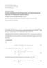
- 6 EURASIP Journal on Advances in Signal Processing 101 102 100 101 10−1 100 Mean square deviation Mean square deviation 10−2 10−1 10−3 10−2 10−4 10−3 10−5 10−4 10−6 10−5 10−7 10−6 0 2000 4000 6000 8000 10000 0 2000 4000 6000 8000 10000 Number of iterations Number of iterations Q=1 Q=3 Q=1 Q=4 Q=2 Q=4 Q=2 Ref. [17] Q=3 Figure 2: Mean square deviation learning curve of the proposed algorithm for varying constraint. Figure 3: Mean square deviation learning curves of the proposed algorithm for varying constraint and a colored input signal. of feedback, M the number of feedforward coefficients H2 (z) for the linear subsystem, and L the number of coef- 1.0000 − 1.8000z−1 +1.6200z−2 − 1.4580z−3 +0.6561z−4 = ficients for the polynomial subsystem. Based on these , 1.0000 − 0.2314z−1 +0.4318z−2 − 0.3404z−3 +0.5184z−4 coefficient numbers, let K represent N + M + L − 2 (47) in the computation of the computational cost of our proposed adaptive nonlinear algorithm. In computing the and static nonlinearity modeled as a polynomial with computational cost, we assume that the cost of invert- coefficients ing a K × K matrix is (K 3 ) (Multiplications and (L2 N ) for computing R−1 [28]. Under additions) and z(n) = x(n) − 0.3x(n)2 + 0.2x(n)3 . (48) these assumptions, the computational cost of our pro- posed algorithm is of (QK 2 ) multiplications compared The desired response signal d(n) of the adaptive Ham- (K 2 ) in [17]. This increase in complexity due to to merstein filter was obtained by corrupting the output of the the order of the input regression matrix in the proposed unknown system with additive white noise of zero mean algorithm is compensated for by the algorithms good and variance such that the output signal to noise ratio was performance. 30 dB. The proposed algorithm was initialized as follows: λn = 0.997, μopt = 1.5e − 6, δ = 5e − 4, and C = 0.0001. Figure 2 shows the mean square deviation between the 4. Simulation Results estimated and optimum Hammerstein filter weights for a white input case. The results were obtained, by ensemble In this section, we validate the proposed algorithm with averaging over 100 independent trials. The figure shows simulation results corresponding to two different types of that the convergence speed of the proposed algorithm is input signals (white and highly colored signals). The white directly correlated to the number of constraints Q used in signal was an additive white Gaussian noise signal of zero the algorithm. mean and unity variance. The highly colored signal was Figure 3 shows a comparison of the mean square devia- generated by filtering the white signal with a filter of tion learning curve obtained, from the proposed algorithm impulse response: and the algorithm in [17]. The proposed algorithm outper- formed [17] even though the authors had used the Gram Schmidt process to better enhance the algorithms perfor- 0.5 H1 (z) = mance in a colored environment. This result is expected since . (46) 1 + 0.9z−1 [17] is sensitive to the additional step-size and regularizing parameters that govern the adaptation of the Gram-Schmidt The Hammerstein system was modeled such that the processor. Results also show that, above a constraint value dynamic linear system had an impulse response H2 (z) of 1 (Q > 1), the proposed algorithms performance in the given by colored environment is similar.
- EURASIP Journal on Advances in Signal Processing 7 5. Conclusion [15] J. V¨ r¨ s, “Iterative algorithm for parameter identification of oo Hammerstein systems with two-segment nonlinearities,” IEEE We have proposed a new adaptive filtering algorithm for Transactions on Automatic Control, vol. 44, no. 11, pp. 2145– the Hammerstein model filter based on the theory of Affine 2149, 1999. Projections. The new algorithm minimizes the norm of the [16] E.-W. Bai, “An optimal two-stage identification algorithm for projected weight error vector as a criterion to track the Hammerstein-Wiener nonlinear systems,” Automatica, vol. 34, no. 3, pp. 333–338, 1998. adaptive Hammerstein algorithm’s optimum performance. Simulation results confirm the convergence of the parameter [17] J. Jeraj and V. J. Mathews, “A stable adaptive Hammerstein fil- ter employing partial orthogonalization of the input signals,” estimates from our proposed algorithm to its corresponding IEEE Transactions on Signal Processing, vol. 54, no. 4, pp. 1412– parameter in the plants parameter vector. 1420, 2006. [18] E.-W. Bai, “A blind approach to the Hammerstein-Wiener References model identification,” Automatica, vol. 38, no. 6, pp. 967–979, 2002. [1] T. Ogunfunmi, Adaptive Nonlinear System Identification: [19] I. J. Umoh and T. Ogunfunmi, “An adaptive algorithm for Volterra and Wiener Model Approaches, Springer, London, UK, Hammerstein filter system identification,” in Proceedings of the 2007. 16th European Signal Processing Conference (EUSIPCO ’08), [2] V. J. Mathews and G. L. Sicuranza, Polynomial Signal Process- Lausanne, Switzerland, August 2008. ing, John Wiley & Sons, New York, NY, USA, 2000. [20] F. Ding, T. Chen, and Z. Iwai, “Adaptive digital control of [3] T. Ogunfunmi and S. L. Chang, “Second-order adaptive Hammerstein nonlinear systems with limited output sam- Volterra system identification based on discrete nonlinear pling,” SIAM Journal on Control and Optimization, vol. 45, no. Wiener model,” IEE Proceedings: Vision, Image and Signal 6, pp. 2257–2276, 2007. Processing, vol. 148, no. 1, pp. 21–30, 2001. [21] V. J. Mathews and Z. Xie, “Stochastic gradient adaptive filter [4] S.-L. Chang and T. Ogunfunmi, “Stochastic gradient based with gradient adaptive step size,” IEEE Transactions on Signal third-order Volterra system identification by using nonlinear Processing, vol. 41, no. 6, pp. 2075–2087, 1993. Wiener adaptive algorithm,” IEE Proceedings: Vision, Image [22] A. Benveniste, M. Metivier, and P. Priouret, Adaptive Algo- and Signal Processing, vol. 150, no. 2, pp. 90–98, 2003. rithms and Stochastic Approximation, Springer, New York, NY, [5] W. Greblicki, “Nonlinearity estimation in Hammerstein sys- USA, 1990. tems based on ordered observations,” IEEE Transactions on [23] D. P. Mandic, “A generalized normalized gradient descent Signal Processing, vol. 44, no. 5, pp. 1224–1233, 1996. algorithm,” IEEE Signal Processing Letters, vol. 11, no. 2, part [6] S. Prakriya and D. Hatzinakos, “Blind identification of linear 1, pp. 115–118, 2004. subsystems of LTI-ZMNL-LTI models with cyclostationary [24] S. Haykin, Adaptive Filter Theory, Prentice-Hall, Upper Saddle inputs,” IEEE Transactions on Signal Processing, vol. 45, no. 8, River, NJ, USA, 4th edition, 2002. pp. 2023–2036, 1997. [25] N. J. Bershad, “On the optimum data nonlinearity in LMS [7] K. J. Hunt, M. Munih, N. N. de Donaldson, and F. M. D. adaptation,” IEEE Transactions on Acoustics, Speech, and Signal Barr, “Investigation of the hammerstein hypothesis in the Processing, vol. 34, no. 1, pp. 69–76, 1986. modeling of electrically stimulated muscle,” IEEE Transactions [26] A. Carini, V. John Mathews, and G. L. Sicuranza, “Sufficient on Biomedical Engineering, vol. 45, no. 8, pp. 998–1009, 1998. stability bounds for slowly varying direct-form recursive linear [8] D. T. Westwick and R. E. Kearney, Identification of Nonlinear filters and their applications in adaptive IIR filters,” IEEE Physiological Systems, John Wiley & Sons, New York, NY, USA, Transactions on Signal Processing, vol. 47, no. 9, pp. 2561–2567, 2003. 1999. [9] S. W. Su, L. Wang, B. G. Celler, A. V. Savkin, and Y. [27] C. R. Johnson Jr., “Adaptive IIR filtering: current results and Guo, “Identification and control for heart rate regulation open issues,” IEEE Transactions on Information Theory, vol. 30, during treadmill exercise,” IEEE Transactions on Biomedical no. 2, pp. 237–250, 1984. Engineering, vol. 54, no. 7, pp. 1238–1246, 2007. [28] J. M. Cioffi and T. Kailath, “Fast, recursive-least-squares [10] D. P. Mandic and J. A. Chambers, Recurrent Neural Networks transversal filters for adaptive filtering,” IEEE Transactions on for Prediction: Learning Algorithms, Architectures and Stability, Acoustics, Speech, and Signal Processing, vol. 32, no. 2, pp. 304– John Wiley & Sons, Chichester, UK, 2001. 337, 1984. [11] F. Ding, Y. Shi, and T. Chen, “Auxiliary model-based least- squares identification methods for Hammerstein output-error systems,” Systems and Control Letters, vol. 56, no. 5, pp. 373– 380, 2007. [12] E.-W. Bai, “Identification of linear systems with hard input nonlinearities of known structure,” Automatica, vol. 38, no. 5, pp. 853–860, 2002. [13] F. Giri, F. Z. Chaoui, and Y. Rochdi, “Parameter identification of a class of Hammerstein plants,” Automatica, vol. 37, no. 5, pp. 749–756, 2001. [14] M. Boutayeb, H. Rafaralahy, and M. Darouach, “A robust and recursive indentificaition method for Hammerstein model,” in Proceedings of the IFAC World Congress, pp. 447–452, San Francisco, Calif, USA, 1996.
CÓ THỂ BẠN MUỐN DOWNLOAD

-

Báo cáo hóa học: "Research Article Are the Wavelet Transforms the Best Filter Banks for Image Compression?"
 7 p |
7 p |  120
|
120
|  7
7
-

Báo cáo hóa học: "Research Article Detecting and Georegistering Moving Ground Targets in Airborne QuickSAR via Keystoning and Multiple-Phase Center Interferometry"
11 p | 116
| 7
-

Báo cáo hóa học: "Research Article Cued Speech Gesture Recognition: A First Prototype Based on Early Reduction"
19 p | 116
| 6
-

Báo cáo hóa học: " Research Article Practical Quantize-and-Forward Schemes for the Frequency Division Relay Channel"
11 p | 114
| 6
-

Báo cáo hóa học: " Research Article Breaking the BOWS Watermarking System: Key Guessing and Sensitivity Attacks"
8 p | 104
| 6
-

Báo cáo hóa học: "Research Article Application-Specific Instruction Set Processor Implementation of List Sphere Detector"
14 p | 60
| 6
-

Báo cáo hóa học: " Research Article A Fuzzy Color-Based Approach for Understanding Animated Movies Content in the Indexing Task"
17 p | 108
| 6
-

Báo cáo hóa học: "Research Article Exploring Landmark Placement Strategies for Topology-Based Localization in Wireless Sensor Networks"
12 p | 118
| 5
-

Báo cáo hóa học: " Research Article A Motion-Adaptive Deinterlacer via Hybrid Motion Detection and Edge-Pattern Recognition"
10 p | 93
| 5
-

Báo cáo hóa học: " Research Article Some Geometric Properties of Sequence Spaces Involving Lacunary Sequence"
8 p | 94
| 5
-

Báo cáo hóa học: " Research Article Eigenvalue Problems for Systems of Nonlinear Boundary Value Problems on Time Scales"
10 p | 90
| 5
-

Báo cáo hóa học: "Research Article Color-Based Image Retrieval Using Perceptually Modified Hausdorff Distance"
10 p | 97
| 5
-

Báo cáo hóa học: "Research Article Probabilistic Global Motion Estimation Based on Laplacian Two-Bit Plane Matching for Fast Digital Image Stabilization"
10 p | 112
| 4
-

Báo cáo hóa học: " Research Article An MC-SS Platform for Short-Range Communications in the Personal Network Context"
12 p | 70
| 4
-

Báo cáo hóa học: "Research Article Quantification and Standardized Description of Color Vision Deficiency Caused by"
9 p | 120
| 4
-

Báo cáo hóa học: " Research Article Hilbert’s Type Linear Operator and Some Extensions of Hilbert’s Inequality"
10 p | 77
| 4
-
Báo cáo hóa học: "Research Article On the Generalized Favard-Kantorovich and Favard-Durrmeyer Operators in Exponential Function Spaces"
12 p | 102
| 4
-

Báo cáo hóa học: " Research Article Approximation Methods for Common Fixed Points of Mean Nonexpansive Mapping in Banach Spaces"
7 p | 74
| 3


Chịu trách nhiệm nội dung:
Nguyễn Công Hà - Giám đốc Công ty TNHH TÀI LIỆU TRỰC TUYẾN VI NA
LIÊN HỆ
Địa chỉ: P402, 54A Nơ Trang Long, Phường 14, Q.Bình Thạnh, TP.HCM
Hotline: 093 303 0098
Email: support@tailieu.vn
Giấy phép Mạng Xã Hội số: 670/GP-BTTTT cấp ngày 30/11/2015 Copyright © 2022-2032 TaiLieu.VN. All rights reserved.

