Báo cáo hóa học: " Research Article An Improved Flowchart for Gabor Order Tracking with Gaussian Window as the Analysis Window"

Chia sẻ: Nguyen Minh Thang | Ngày: | Loại File: PDF | Số trang:9

Thêm vào BST

Báo xấu

47
lượt xem 6
download

Download Vui lòng tải xuống để xem tài liệu đầy đủ

Tuyển tập báo cáo các nghiên cứu khoa học quốc tế ngành hóa học dành cho các bạn yêu hóa học tham khảo đề tài: Research Article An Improved Flowchart for Gabor Order Tracking with Gaussian Window as the Analysis Window

Chủ đề:

Bình luận(0) Đăng nhập để gửi bình luận!

Lưu

Nội dung Text: Báo cáo hóa học: " Research Article An Improved Flowchart for Gabor Order Tracking with Gaussian Window as the Analysis Window"

Hindawi Publishing Corporation EURASIP Journal on Advances in Signal Processing Volume 2011, Article ID 507215, 9 pages doi:10.1155/2011/507215 Research Article An Improved Flowchart for Gabor Order Tracking with Gaussian Window as the Analysis Window Yang Jin1, 2 and Zhiyong Hao1 1 Department of Energy Engineering, Power Machinery and Vehicular Engineering Institute, Zhejiang University, Hangzhou 310027, China 2 Department of Automotive Engineering, Hubei University of Automotive Technology, Shiyan 442002, China Correspondence should be addressed to Yang Jin, jin yang@163.com Received 1 July 2010; Revised 21 November 2010; Accepted 19 December 2010 Academic Editor: Antonio Napolitano Copyright © 2011 Y. Jin and Z. Hao. This is an open access article distributed under the Creative Commons Attribution License, which permits unrestricted use, distribution, and reproduction in any medium, provided the original work is properly cited. Based on simulations on the ability of the Gaussian-function windowed Gabor coeﬃcient spectrum to separate order components, an improved ﬂowchart for Gabor order tracking (GOT) is put forward. With a conventional GOT ﬂowchart with Gaussian window, successful order waveform reconstruction depends signiﬁcantly on analysis parameters such as time sampling step, frequency sampling step, and window length in point number. A trial-and-error method is needed to ﬁnd such parameters. However, an automatic search with an improved ﬂowchart is possible if the speed-time curve and order diﬀerence between adjacent order components are known. The appropriate analysis parameters for a successful waveform reconstruction of all order components within a given order range and a speed range can be determined. 1. Introduction (i) It is not suitable for signals with cross-order compo- nents [5]. Because of the inherent mechanism features, the frequency (ii) The appropriate analysis parameters are determined contents of the main excitations in rotary machinery are by the trial-and-error method (human-computer interaction) to separate order components in the integer or fractional multiples of a fundamental frequency, Gabor coeﬃcient spectrum. However, no reports which is usually the rotary speed of the machine [1]. The have explained how to ﬁnd the appropriate param- integer or fractional multiples of the fundamental frequency eters. are called “harmonics” or “orders.” A machine’s run-up or run-down operation is a typical nonstationary process. In this study, we addressed the second limitation, and The excitations in the machine are analogous to frequency- established a ﬂowchart for GOT without trial and error. sweep excitations with several excitation frequencies at a time We ﬁrst generalized the conditions from simulations under which a Gabor coeﬃcient spectrum with a Gaussian window instant because the fundamental frequency is time varying. The vibroacoustic signals acquired during this stage carry can separate order components, and then combined the information about structural dynamics. Information extrac- conditions and current GOT technique for an improved tion from these signals is important. Order tracking (OT) is a ﬂowchart. dedicated nonstationary signal processing technique dealing This paper is organized as follows. Section 2 introduces with rotary machinery. Several computational OT techniques the GOT and the convergence conditions for the recon- have been developed, such as resampling OT [1], Vold- structed order waveform. Section 3 investigates the ability of a Gabor coeﬃcient spectrum with Gaussian window Kalman OT [2, 3], and Gabor OT (GOT) [4], each with its strengths and shortcomings. Among them, GOT can easily to separate order components using simulation. Section 4 implement the reconstruction of order waveforms, but it has explains the improved ﬂowchart. Section 5 veriﬁes the the following limitations. proposed ﬂowchart. Section 6 concludes the paper.
2 EURASIP Journal on Advances in Signal Processing whether h[i] and γ[i] are like. However, the idea behind 2. GOT and the Convergence Conditions for the GOT is to reconstruct the diﬀerent order components (or Reconstructed Order Waveforms harmonics) in the signal. There are three other conditions 2.1. Discrete Gabor Transform and Gabor Expansion. GOT is for the convergence of the reconstructed order waveforms. based on the transform pair of discrete Gabor transform (1) (i) The analysis window γ[i] has to be localized in the and Gabor expansion (2) [6]. Gabor expansion is also called joint time-frequency domain so that cm,n will depict Gabor reconstruction or synthesis: the signal’s time-frequency properties. In the context of rotary machinery, cm,n are desired to describe the mΔM +L/ 2−1 signal’s time-varying harmonics for a run-up or run- ∗ s[i]γm,n [i], cm,n = down signals. i=mΔM −L/ 2 (1) (ii) The time-frequency resolution of γ[i] should be able mΔM +L/ 2−1 − j 2πni/N ∗ to separate adjacent harmonics within the desired s[i]γ [i − mΔM ]e = , order range and rotary speed range. i=mΔM −L/ 2 (iii) The behaviors of h[i] and γ[i], such as time/fre- M −1 N −1 s[i] = cm,n hm,n [i] quency centers and time/frequency resolution, have to be close. Only in this way will the reconstructed m=0 n=0 (2) time waveform with (4) converge to the actual order M −1N −1 component: cm,n h[i − mΔM ]e j 2πni/N , = m=0 n=0 s p [i] where s[i] is the signal, i, m, n, ΔM , M , N , L ∈ Z , ΔM denotes M −1 N −1 M −1 N −1 the time sampling step in the point number; M denotes the cm,n h[i − mΔM ]e j 2πni/N , cm,n hm,n [i] = = time sampling number, N denotes the frequency sampling m=0 n=0 m=0 n=0 number or frequency bins; and L denotes the window (4) length in point number, and “∗” denotes complex conjugate operation. where cm,n denotes the extracted Gabor coeﬃcients asso- The set of the functions {hm,n [i]}m,n∈Z is the Gabor ciated with the desired order p, and s p [i] denotes the elementary functions, also termed as the set of synthetic reconstructed pth order component waveform. functions, and {γm,n [i]}m,n∈Z is the set of analysis functions. Given a window function h[i], the Gabor transform’s h[i] is the synthetic window and γ[i] is the analysis window. time sampling step ΔM , and the frequency sampling step N , Thus, {hm,n [i]}m,n∈Z and {γm,n [i]}m,n∈Z are the time-shifted the orthogonal-like Gabor expansion technique [8], which and harmonically modulated versions of h[i] and γ[i], seeks the optimal dual window so that the dual window respectively. γ[i] most approximates a real-value scaled h[i], has been Equation (1) shows that the Gabor coeﬃcients, cm,n , are developed. When h[i] is the discrete Gaussian function, that the sampled short-time Fourier transform with the window is, function γ[i]. To utilize the FFT, the frequency bin, N , is set to be equal to L, which has to be a power of 2. L has LL 1 D2 e−1/4(i/σ ) h[i] = g [i] = ∀i ∈ − , −1 , 4 to be divided by both N and ΔM in view of numerical 2π (σ D )2 22 implementation. For stable reconstruction, the oversampling (5) rate deﬁned by then when N ΔM · N ros = (3) 2 2 σD D = σopt ΔM = (6) , 4π must be greater or equal to one. It is called the critical the obtained dual window by the orthogonal-like technique sampling rate when γos equals one. The critical sampling is the optimal [7]. Moreover, the optimal dual window is means the number of Gabor coeﬃcients is equal to the related to the oversampling rate. Generally, the diﬀerence number of signal samples. between a window and its optimal dual window decreases Equation (2) exists if and only if h[i] and γ[i] form a as the oversampling rate increases. The diﬀerence between pair of dual functions [7]. Their positions in (1) and (2) are the analysis and synthesis windows is negligible for the interchangeable. commonly used window functions, such as the Gaussian and Hanning windows when the oversampling rate is not less than four [7]. The window in this study is limited to the 2.2. Convergence Conditions for Reconstructed Order Wave- Gaussian window. forms. Given h[i], ΔM and N , generally, the solution of γ[i] is not unique. If viewed only from pure mathematics, we can perfectly reconstruct the signal s[i] with (1) and (2) as long 2.3. Conventional Flowchart for GOT. Figure 1 is the ﬂow- as γos ≥ 1 and γ[i] is a dual function of h[i], regardless chart for the conventional GOT routine. There is no
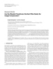
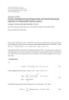
EURASIP Journal on Advances in Signal Processing 3 Begin Select L, N , ΔM N ≥ 4, mod L, N = 0, mod L, ΔM = 0 ΔM Calculate the optimal time standard deviation of ΔM · N 2 D the discrete Gaussian window: σopt = 4π Generate the synthetic window: 2 i/σ D − 1/ 4 1 h[i] = g [i] = 2e 4 2π σ D LL i∈ − , −1 22 Calculate the analysis window γ[i] Adjust L, N , ΔM Calculate cm,n with (1) and plot ˜ the Gabor coeﬃcient spectrum |cm,n | ˜ Can |cm,n | separate ˜ No the order components of interest? Yes Extract the Gabor coeﬃcients cm,n , which ^ are associated with a desired order p Reconstruct the desired order waveform with (4) Perform further analysis to ^p (i) s End (mod(x, y ) denotes computing the remainder of x/ y ) Figure 1: Flowchart for the conventional GOT. 3. Simulation Investigation on the Ability of the problem about the convergence conditions (1) and (3), while condition (2) is satisﬁed using the trial-and-error Gabor Coefﬁcient Spectrum with Gaussian method. Window to Separate Order Components In conventional GOT ﬂowcharts, human-computer in- To examine the ability of the Gabor coeﬃcient spectrum teraction is needed to determine the appropriate analysis parameters. Each time the analysis parameters are changed, to separate order components quantitatively, the Gaussian the user needs to give a visual inspection to the obtained window, which is optimally localized in the time-frequency Gabor coeﬃcient spectrum to judge how well the order domain, is used as the analysis window. The time standard deviation σt in seconds of the Gaussian window in the components are separated in the spectrum. If it fails, then the analysis parameters are adjusted to get another Gabor continuous time domain is utilized as an input parameter to coeﬃcient spectrum. generate the discrete window in discrete Gabor transform. Its
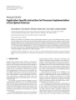
4 EURASIP Journal on Advances in Signal Processing advantage is that it is easy to ﬁnd the relationship between σt seconds and the ordinate is frequency in Hz. The color in the spectrum indicates the magnitude of the Gabor coeﬃcients. and the signal’s characteristic because the signals of interest S1 consists of ﬁve order components and a Gaussian come originally from the continuous time domain. white noise with SNR equal to 50 (34 dB). The rotary speed n = 60t ; the instantaneous amplitude of the pth order 3.1. The Gaussian Window and Its Time Standard Deviation. component A p (t ) = 1; the instantaneous frequency of the The energy-normalized discrete Gaussian window is pth order component f p (t ) = p · t . The closer two components are located theoretically 1 1 2 −1/ 4(i/σ D ) 2 −1/ 4(i/ (σt fs )) g [i] = 2e 2e = 4 in the time-frequency domain, the more likely they will 4 2π (σ D ) 2π σt fs overlap in the Gabor coeﬃcient spectrum and the more diﬃcult it will be to distinguish them. The feature of run- 1 up or run-down signals is that not only are there multiple 2 −L2 / (4σt2 fs2 )(i/L) 2e = 4 2π σt fs components at the same time instant but there are also multiple components at the same frequency. In Figure 2(a), at 6.82 s (indicated by line “0”), the LL 1 2 −1/ (4σN 2 )(i/L) 2e ∀i ∈ − , = −1 , 4 frequency spacing between the adjacent order components 2π σt fs 22 is 6.82 Hz, equal to 6σ f . There are no obvious overlaps (7) between the ﬁve components at times larger than 6.82 s. When the time is larger than 6.82 s, the theoretical time where fs denotes sampling frequency, L denotes the window spacing between any adjacent two-order components at the length in point number, σ D denotes the standard deviation same frequency is larger than 6σt . of the discrete window, and σt denotes the time standard When σt is equal to 200 ms, 6σ f is equal to 2.387 Hz deviation in seconds of the continuous time domain function (Figure 2(b)), and the instantaneous frequency spacing g (t ), whose sampled version is g[i]: between the adjacent order components is larger than 6σ f when the time is larger than 2.387 s. However, diﬀerent from σD σt = Figure 2(a), there are still overlaps in Figure 2(b) between , (8) fs the components when the time is larger than 2.387 s. These are due to the small time spacing between the adjacent where σN denotes a normalized value deﬁned by order components at the same frequency. The overlaps exist between S4 and S5 below the frequency of about 24 Hz, at σt f s σN = . which the corresponding instant of S4 is 6 s and that of S5 is (9) L 4.8 s. The spacing is 1.2 s, equal to 6σt . Similarly, the overlaps exist between S4 and S3 below the frequency of about 14.4 Hz, Window length L should be large enough to make σN where the corresponding time of S3 is 4.8 s, and that of S4 is small enough. Small σN means the values at both ends of the 3.6 s. The spacing is 1.2 s, also equal to 6σt . We can explain Gaussian window are small, which will reduce the spectral leakage in Gabor transform. In our simulations, σN ≤ 0.1 Figure 2(c) in a similar manner. To sum up, assume that fspaing,min (Hz) is the minimum was generally guaranteed, which implies that the values at theoretical frequency spacing between the adjacent order both ends of the Gaussian window are not larger than 0.2% components at the same time instant and tspacing,min (s) is of the window’s peak value. the minimum theoretical time spacing between the adjacent The frequency domain standard deviation in Herzs of g (t ) is order components at the same theoretical frequency. If a Gabor coeﬃcient spectrum with a Gaussian window of time standard width σt can separate the order components within 1 σf = . (10) 4πσt a given order range and a speed range (i.e., the coeﬃcient at any time-frequency sampling point is signiﬁcantly the contribution from an individual component but not a 3.2. Simulations. The discrete Gabor transform (1) is no combined contribution of several adjacent components), more than a sampled short-time Fourier transform (STFT). then there are the following approximate relationships: The inherent limitation of STFT is that its time and frequency resolutions cannot be improved simultaneously. Our simulations did not aim to demonstrate this point but 6 6 fspacing,min ≥ 6σ f = ⇐ σt ≥ σt,min = ⇒ , to disclose the conditions under which the Gabor coeﬃcient 4πσt 4π fspacing,min spectrum can separate order components. We limited the (11) frequency bins N equal to L. tspacing,min Figure 2 depicts three Gabor coeﬃcient spectra of tspacing,min ≥ 6σt ⇐⇒ σt ≤ σt,max = . (12) the simulation signal S1 with diﬀerent Gaussian window 6 functions. For convenience of explanation, auxiliary points “0,” “1,” some auxiliary lines, and two characteristic values Inequalities (11) and (12) are the conditions for the min- determined from numerical experiments, 6σ f and 6σt , are imum frequency spacing and the minimum time spacing, listed in this ﬁgure. In each spectrum, the abscissa is time in respectively.
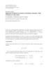
EURASIP Journal on Advances in Signal Processing 5 45 45 8.409 6.912 S5 0 40 40 S4 6 1.2 s 1.2 s S3 35 35 6 Frequency (Hz) Frequency (Hz) 30 30 4 S2 25 25 |cm,n | |cm,n | 24 Hz 4 ˜ ˜ 20 20 15 15 S1 14.4 Hz 2 2 10 10 5 5 0 0 0 2 4 6 8 10 12 15 2 4 6 8 10 12 15 Time (s) Time (s) σt = 70 ms fs = 200 Hz σt = 200 ms fs = 200 Hz 6σt = 420 ms L = 2048 6σt = 1.2 s L = 2048 6σ f = 6.82 Hz ΔM = 2 6σ f = 2.387 Hz ΔM = 2 σN = 0.0068 σN = 0.0195 (a) (b) 60 7.383 2.04 s 2.04 s 50 6 Frequency (Hz) 40.8 Hz 40 |cm,n | 4 30 ˜ 24.48 Hz 20 2 10 0 2 4 6 8 10 12 15 Time (s) σt = 340 ms fs = 200 Hz 6σt = 2.04 s L = 2048 6σ f = 1.404 Hz ΔM = 2 σN = 0.0332 (c) 5 Figure 2: Gabor coeﬃcient spectra with diﬀerent Gaussian window widths for Signal S1, S1(t ) = S p (t ) + Noise|SNR=50(34 dB) = p=1 5 p=1 cos(2π p(t / 2)) + Noise|SNR=50(34 dB) . 2 4. Improved GOT Flowchart The smaller the rotary speed and the larger the order, the smaller the time spacing between adjacent order components A Gabor coeﬃcient spectrum that could separate the order at the same frequency and the more liable the destruction components is obtained by trial and error in the conventional of the condition for the minimum time spacing. It can be GOT ﬂowchart. The conditions for σt ((11) and (12)) to determined from Figure 4 that separate components in the Gabor coeﬃcient spectrum are nmin · Δ p used to improve the GOT ﬂowchart (Figure 3). Determining tspaing,min = tB = , (13) pmax · k fspaing,min and tspacing,min becomes the ﬁrst step in the improved ﬂowchart, and σt is then determined by (11) and nmin · Δ p fspacing,min = . (12) to generate the Gaussian window (analysis window). It (14) 60 is possible that there is no value for σt that could separate all order components within a given order and a speed range. Equtions (13) and (14) hold when the speed is linearly varying and the order diﬀerence between the adjacent order 4.1. Determination of fspacing,min and tspacing,min . Given a components is the same. When the speed does not change Gaussian window’s σt for discrete Gabor transform, when the this way, it is still easy to determine fspacing,min analytically. order diﬀerence between the adjacent order components are fspacing,min = (nmin / 60)Δ pmin , where Δ pmin denotes the minimum order diﬀerence between the adjacent order the same (Figure 4), it is liable to destroy the condition for components. However, it would be diﬃcult to determine the minimum frequency spacing with a small rotary speed.
6 EURASIP Journal on Advances in Signal Processing Begin Within desired speed range and order range determine tspacing,min , fspacing,min Determine σt,min , σt,max with (11), (12) No σt,max ≥ σt,min ? Yes Choose a value in [σt,min , σt,max ] ⇒ σt There exits no appropriate σt to realize the waveform reconstruction of all order components within the desired order and speed ranges. It is Select L to satisfy σN ≤ 0.1 possible when the maximum order of interest is reduced or L⇒N the lowest speed is increased. Generate the Gaussian window g [i] with (7); g [i] ⇒ γ[i] According to (6) and (8), 4πσt2 fs2 ⇒ ΔM Round2 L (Round2 x denotes rounding x to a power of 2 that is not larger than x) Calculate the dual window h[i] Calculate cm,n with (1) and plot ˜ the Gabor coeﬃcient spectrum |cm,n | ˜ Extract the Gabor coeﬃcients cm,n , which ^ are associated with a desired order p Reconstruct the order waveform with (4) Perform further analysis to ^p (i) s End Figure 3: Flowchart for the improved GOT. tspacing,min analytically even if it is not impossible. However, f j (t ), j = 0, 1, . . . J , (15) as long as the speed n(t ) changes monotonously, we can of all order components according to the speed-time curve numerically determine tspacing,min within the given speed n(t ), where j denotes the index for the order value p j range [nmin , nmax ], order range [ pmin , pmax ], and frequen- within [ pmin , pmax ] and j increases as p j increases; the order cy range [ fmin , fmax ]. The process is described as follows diﬀerence between the adjacent order components Δ p j | j ≥1 = (Figure 5): p j − p j −1 , (iii) i = 0, fi = fmin , (i) input n(t ), [nmin , nmax ], [ pmin , pmax ], [ fmin , fmax ], δ f , (iv) ﬁnd the abscissa t j of the intersection of the two curves: f (t ) = fi and f (t ) = f j (t ), j = 1, 2, . . . , J , (ii) calculate the theoretical frequency curve
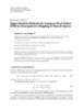
EURASIP Journal on Advances in Signal Processing 7 pmax + Δ p order tspacing,min pmax order A(0, ( pmax + Δ p)nmin / 60) B(tB , pmax (nmin + k · tB )/ 60) Frequency (Hz) fspacing,min 0 Time (s) Rotary speed: n = nmin + k · t nmin (r/ min): the lowest rotary speed pmax : the highest order of interest in a signal Δ p: the order diﬀerence between adjacent order components k (r/ (min · s)): the change rate of the rotary speed Figure 4: Schematic diagram for the theoretical time-frequency locations of order components in a signal with linearly increasing speed. fmax . . . Frequency (Hz) f j (t ), p j order fi f j −1 (t ), p j −1 order f j −2 (t ), p j −2 order . . . fmin tspacing, j tspacing, j −1 tj t j −1 t j −2 Time (s) Figure 5: Schematic diagram for searching for tspacing,min . 30th order 25th order 600 19.444 550 15 Frequency (Hz) 500 |cm,n | 10 ˜ 450 n(t ) (r/min) 50 1800 5 400 30 1400 S2(t ) 10 1000 −10 0.1011 350 600 0 1 2 3 4 5 6 7 8 9 0 1 3 5 7 9 Time (s) Time (s) σt = 40 ms fs = 8192 Hz 6σt = 240 ms L = 4096 6σ f = 11.93 Hz ΔM = 256 σN = 0.08 (b) (a) Figure 6: The Gabor coeﬃcient spectrum of the simulation signal S2(t ) based on the improved ﬂowchart. (a) Gabor coeﬃcient spectrum of signal S2(t ); and (b) signal S2(t ) (in black) and the simultaneous speed n(t ) (in red).
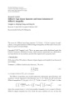
8 EURASIP Journal on Advances in Signal Processing 700 21.226 20.5th order 600 500 15 Frequency (Hz) 16.5th order 400 |cm,n | 10 ˜ 300 200 n(t ) (r/min) 10 2100 5 2nd order 1900 S3(t ) 100 0 1700 −5 0 0.0003 −10 1500 4.227 6 10 14 18 21.135 4.227 6 10 14 18 21.135 Time (s) Time (s) σt = 80 ms fs = 2048 Hz 6σt = 480 ms L = 2048 6σ f = 5.968 Hz ΔM = 128 σN = 0.08 (b) (a) Figure 7: The Gabor coeﬃcient spectrum of an actual signal S3(t ) based on the improved ﬂowchart. (a) Gabor coeﬃcient spectrum of signal S3(t ); and (b) signal S3(t ) (in black) and the simultaneous speed n(t ) (in red). 1.4 1000 1.25 17th order 16th order 800 1 Frequency (Hz) 600 12th order |cm,n | 0.75 8th order ˜ 400 0.5 n(t ) (r/min) 0.6 4000 200 0.25 0.2 3000 S4(t ) −0.2 2000 4th order −0.6 0 0 1000 0.773 2 4 6 8 10 11.237 0.773 2 4 6 8 10 11.237 Time (s) Time (s) σt = 37 ms fs = 4 kHz 6σt = 222 ms L = 2048 6σ f = 12.9 Hz ΔM = 128 σN = 0.0723 (b) (a) Figure 8: The Gabor coeﬃcient spectrum of an actual signal S4(t ) based on the improved ﬂowchart. (a) Gabor coeﬃcient spectrum of signal S4(t ); and (b) signal S4(t ) (in black) and the simultaneous speed n(t ) (in red). (ix) ﬁnd the minimum of the set {tspacing,i } and assign it (v) to tspacing,min . ⎧ ⎪ t j − t j −1 if both t j and t j −1 exist , ⎨ tspacing, j = ⎪ 5. Veriﬁcation ⎩ if neither t j nor t j −1 exists , ∞ To verify the eﬀectiveness of the improved ﬂowchart, a j = 1, 2, . . . , J , simulation signal is deﬁned as (16) 40 S2(t ) = S p + Noise|SNR=50(34 dB) (vi) ﬁnd the minimum of the set {tspacing, j } j ≥1 and assign p=1 it to tspacing,i , 40 2π p k (17) A p cos nmin t + t 2 = (vii) i = i + 1, fi = fi + δ f , 60 2 p=1 (viii) repeat steps (4)−(7) until fi is larger than or equal to + Noise|SNR=50(34 dB) , fmax ,
EURASIP Journal on Advances in Signal Processing 9 where nmin = 800 r/ min, k = 93.3 r/ (min ×s); the instan- by a tachometer, and Δ p j can come from prior knowledge taneous amplitude of the pth order component is: about the test objects or be determined by preliminary trials. For the GOT of signals without simultaneous speed A p = 1. (18) information, automatic search of appropriate processing parameters should deserve future research. For this signal, if the order range of interest is [1, 30] and the speed range of interest is above 800 r/min, then fspaing,min References and tspacing,min determined with (13) and (14) are 13.3 Hz and 285.6 ms, respectively. Consequently the appropriate range [1] S. Gade, H. Herlufsen, H. Konstantin-Hansen et al., “Order for σt is [35.8, 47.6] ms. Figure 6 shows the result when σt tracking analysis,” Technical Review 2, Br¨ el & Kjær, 1995. u equals to 40 ms. There are no overlaps between the order [2] S. Gade, H. Herlufsen, H. Konstantin-Hansen et al., “Char- components with an order not larger than 30 in Figure 6(a). acteristics of the Vold-Kalman order tracking ﬁlter,” Technical We tested some real-world signals with simultaneous Review 1, Br¨ el & Kjær, 1999. u [3] M. C. Pan and C. X. Wu, “Adaptive Vold-Kalman ﬁltering order speeds not linearly varying. Figures 7 and 8 are two such tracking,” Mechanical Systems and Signal Processing, vol. 21, no. examples. In both cases, a photoelectric tachometer was used 8, pp. 2957–2969, 2007. to detect the simultaneous speed. [4] S. Qian, “Gabor expansion for order tracking,” Sound and For signal S3(t ) (Figure 7), the order diﬀerence between Vibration, vol. 37, no. 6, pp. 18–22, 2003. the adjacent order components is 0.5, the ranges of interest [5] M. C. Pan, S. W. Liao, and C. C. Chiu, “Improvement on are order range: [0.5, 20], speed range: [1, 600, 2, 100] Gabor order tracking and objective comparison with Vold- r/min; frequency range: [0, 700] Hz. Then fspaing,min with (13) Kalman ﬁltering order tracking,” Mechanical Systems and Signal is 13.3 Hz and tspacing,min determined by numerical algorithm Processing, vol. 21, no. 2, pp. 653–667, 2007. is 511.745 ms, which is between order 20.5 and order 20 at [6] H. Shao, W. Jin, and S. Qian, “Order tracking by discrete the 674 Hz frequency. Consequently, the determined range Gabor expansion,” IEEE Transactions on Instrumentation and for σt with (11) and (12) is [35.8, 85.3] ms. Figure 7 shows Measurement, vol. 52, no. 3, pp. 754–761, 2003. the result when σt equals 80 ms. All order components with [7] S. Qian, Introduction to Time-Frequency and Wavelet Trans- forms, Prentice Hall, Upper Saddle River, NJ, USA, 2002. an order not larger than 20 are separated in Figure 7(a). For signal S4(t ) (Figure 8), the order diﬀerence between [8] S. Qian and D. Chen, “Optimal biorthogonal analysis window function for discrete Gabor transform,” IEEE Transactions on the adjacent order components is 1, the ranges of interest are Signal Processing, vol. 42, no. 3, pp. 694–697, 1994. order range: [1, 16], speed range: [1, 120, 3, 800] r/min, and frequency range: [0, 1, 000] Hz. Then fspaing,min with (13) is 18.7 Hz and tspacing,min determined by numerical algorithm is 219.382 ms, which is between orders 17 and 16 at the 340 Hz frequency. Consequently, the determined range for σt with (11) and (12) is [25.6, 36.6] ms. Figure 8 shows the result when σt equals 36 ms. All order components with an order not larger than 16 are well separated in Figure 8(a). Our tests on simulation and real-world signals indicate that the proposed search of parameters for GOT is successful. 6. Conclusion In this study, we designed an automatic search method to ﬁnd appropriate analysis parameters for GOT, which eliminates the trial-and-error process. We ﬁrst generalized the conditions for the minimum time spacing limit and the minimum frequency spacing limit from simulations, under which the Gabor coeﬃcient spectrum with Gaussian window will well separate order components. The conditions were then utilized to generate an analysis window in the improved GOT ﬂowchart. Our simulation results and real applications both veriﬁed its eﬀectiveness. According to the improved ﬂowchart, as long as σt,min ≤ σt,max , any value within [σt,min , σt,max ] for σt will guarantee well-separated order components in the Gabor coeﬃcient spectrum. This is an important convergence condition for the reconstructed order waveform. The prerequisite for this improved GOT is with a proper speed-time curve and prior knowledge on order diﬀerences between adjacent order components. Usually, the simultaneous speed-time curve is easy to acquire