Báo cáo hóa học: "Research Article Application of Frequency Diversity to Suppress Grating Lobes in Coherent MIMO Radar with Separated Subapertures"

Chia sẻ: Linh Ha | Ngày: | Loại File: PDF | Số trang:10

Thêm vào BST

Báo xấu

70
lượt xem 4
download

Download Vui lòng tải xuống để xem tài liệu đầy đủ

Tuyển tập báo cáo các nghiên cứu khoa học quốc tế ngành hóa học dành cho các bạn yêu hóa học tham khảo đề tài: Research Article Application of Frequency Diversity to Suppress Grating Lobes in Coherent MIMO Radar with Separated Subapertures

Chủ đề:

Bình luận(0) Đăng nhập để gửi bình luận!

Lưu

Nội dung Text: Báo cáo hóa học: "Research Article Application of Frequency Diversity to Suppress Grating Lobes in Coherent MIMO Radar with Separated Subapertures"

Hindawi Publishing Corporation EURASIP Journal on Advances in Signal Processing Volume 2009, Article ID 481792, 10 pages doi:10.1155/2009/481792 Research Article Application of Frequency Diversity to Suppress Grating Lobes in Coherent MIMO Radar with Separated Subapertures Long Zhuang and Xingzhao Liu Department of Electronic Engineering, Shanghai Jiao Tong University, Shanghai 200240, China Correspondence should be addressed to Xingzhao Liu, xzhliu@sjtu.edu.cn Received 5 June 2008; Revised 27 December 2008; Accepted 1 May 2009 Recommended by Ioannis Psaromiligkos A method based on frequency diversity to suppress grating lobes in coherent MIMO radar with separated subapertures is proposed. By transmitting orthogonal waveforms from M separated subapertures or subarrays, M receiving beams can be formed at the receiving end with the same mainlobe direction. However, grating lobes would change to diﬀerent positions if the frequencies of the radiated waveforms are incremented by a frequency oﬀset Δ f from subarray to subarray. Coherently combining the M beams can suppress or average grating lobes to a low level. We show that the resultant transmit-receive beampattern is composed of the range-dependent transmitting beam and the combined receiving beam. It is demonstrated that the range-dependent transmitting beam can also be frequency oﬀset-dependent. Precisely directing the transmitting beam to a target with a known range and a known angle can be achieved by properly selecting a set of Δ f . The suppression eﬀects of diﬀerent schemes of selecting Δ f are evaluated and studied by simulation. Copyright © 2009 L. Zhuang and X. Liu. This is an open access article distributed under the Creative Commons Attribution License, which permits unrestricted use, distribution, and reproduction in any medium, provided the original work is properly cited. 1. Introduction A hybrid processing mode for MIMO radar with separated antennas has been proposed in [14, 15]. The authors pointed out that the locations of targets can be Unlike a traditional phased-array radar system, which can previously determined within a limited area by non-coherent only transmit scaled versions of a single waveform, a processing. Then, by coherent processing the resolution can multi-input multi-output (MIMO) radar system has shown be improved to resolve targets located in the same range much ﬂexibility by transmitting multiple orthogonal (or cell. It is demonstrated that by phase synchronizing across incoherent) waveforms [1–15]. The waveforms can be the sparse antennas, the resolution of MIMO radar can be extracted at the receiving end by a set of matched ﬁlters. improved to the level of the carrier wavelength λ0 . However, Each of the extracted components contains the information as also stated in [14, 15], the high resolution mode enabled of an individual transmit-receive path. According to the by the coherent processing of sparse antennas creates grating processing modes for using this information, the MIMO lobes stemming from the large separation between antennas. radars can be divided into two classes. One class is non- To avoid ambiguity in target localization, it is necessary to coherent processing to overcome the radar cross section suppress the unwanted grating lobes to a low level. Randomly (RCS) ﬂuctuation of the target [1–3]. In this scheme, the positioning the antennas can break up the grating lobes at transmitting antennas are separated from each other to ensure that a target is observed from diﬀerent aspects. The the cost of higher sidelobes [16, 17]. The statistical analysis of sidelobes in coherent processing sparse MIMO radar other class is coherent processing [4–13], where the receiving with randomly positioned antennas has been studied in antennas are closely spaced to avoid ambiguity. By using diﬀerent phase shifts associated with diﬀerent propagation [18]. Inspired by using frequency diversity to suppress grating paths, a better spatial resolution can be obtained. Some of the lobes in conventional sparse arrays [19–21], in this paper, we recent work on this class MIMO radar has been reviewed in propose a frequency diverse method to suppress grating lobes [13].
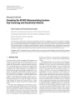
2 EURASIP Journal on Advances in Signal Processing Target transmitted by the ith subarray, and wm [k] is the additive noise at the mth subarray. Aim (θ ) reﬂects the phase shift from Y the ith transmitting subarray to the mth receiving subarray, that is, Aim (θ ) = exp − j 2π f0 (τi (θ ) + τm (θ )) , i, m = 1, . . . , M , θ (2) where f0 is the operating frequency. For all the M transmitted waveforms, there are M × M phase shifts in the receiving sparse array. By combining all the phase shifts, the sparse MIMO aperture array response can be written as X L A(θ ) = a(θ )aT (θ ), Figure 1: MIMO radar with separated subapertures. a(θ ) = asub (θ ) ⊗ aF (θ ), 2π f0 (3) aF (θ ) = 1, exp − j L sin θ , . . . , in sparse MIMO aperture radar systems. We focus on mono- c static sparse MIMO radar, that is, each antenna acts as both T 2π f0 transmitter and receiver. Frequency diversity is achieved by exp − j (M − 1)L sin θ , c transmitting orthogonal waveforms with diverse frequencies from each antenna simultaneously. The radiated frequencies where (·)T denotes the transpose operator, ⊗ stands for the are progressively incremented by a frequency oﬀset Δ f . Kronecker operation, and c is the speed of light. By coherently combining the receiving beams formed at In the matrix notation, (1) can be written as diﬀerent frequencies, the grating lobes can be suppressed or averaged to a low level. It is shown that the transmit-receive Y[k] = αA(θ )S[k] + W(k), k = 1, . . . , K , (4) beampattern (BP) of MIMO radar with frequency diversity is composed of the range-dependent transmitting beam and where Y[k], S[k], and W(k) are the received signal, the the combined receiving beam. The range-dependent beam transmitted signal, and the additive noise, respectively. has been studied in [22–24]. We demonstrate that the range- If the output matrix Y in (4) is reorganized into a column dependent beam can also be frequency oﬀset-dependent. vector, the sparse MIMO array response can be written as Precisely steering the transmitting beam can be achieved by aMIMO (θ ) = a(θ ) ⊗ a(θ ). The matched weight vector of the properly selecting a set of frequency oﬀsets. beamformer will be aMIMO (θ0 ) = a(θ0 ) ⊗ a(θ0 ), where θ0 is The remainder of this paper is organized as follows. the target direction of arrival (DOA). This gives rise to the Section 2 describes the basic sparse MIMO aperture signal following transmit-receive BP: model. The BP of MIMO array with frequency diversity and 2 the selection of the frequency oﬀset are derived in Section 3. H GMIMO (θ ) = aMIMO (θ0 )aMIMO (θ ) The simulation results are given in Section 4, and Section 5 2 is the conclusion. aH (θ0 ) ⊗ aH (θ0 ) [a(θ ) ⊗ a(θ )] = (5) 2 2 2. Basic Signal Model for H H = a (θ0 )a(θ ) a (θ0 )a(θ ) Sparse Mimo Aperture Radar 4 = aH (θ0 )a(θ ) , Consider a monostatic sparse MIMO aperture radar system with M separated subarrays. Each subarray is a standard where (·)H stands for the Hermitian operation. uniform linear array (ULA) with N elements. Let asub (θ ) The resultant transmit-receive BP can be viewed as the be the vector response of subarrays, where θ is the azimuth multiplication of the transmitting beam and the receiving angle. For simplicity, suppose that the sparse distance L beam [7, 8]. In this context, the transmitting beam is iden- between two adjacent subarrays is constant (Figure 1). We tical with the receiving beam. Furthermore, the transmit- assume here that the target RCS is frequency independent. receive BP of the MIMO array is equivalent to the two- In the case of a single target at direction θ the signal received way BP of the conventional phased array. There are two by the mth subarray can be described as [7] diﬀerences between a MIMO radar array and a conventional phased array. First, the orthogonal waveforms in a MIMO M ym [k] = α Aim (θ ) · si [k] + wm [k], radar array enable the radiated energy to cover a broad sector, (1) i=1 and there is no scanning at the transmitting end. Second, the forming of the transmit beam in a MIMO radar array can m = 1, . . . , M , k = 1, . . . , K , be implemented at the receiving end by post-processing, and where k is the time index, α is the complex amplitude of the the transmit-receive BP is obtained using only the received received signal, si [k] is the discrete form of the waveform signals.
EURASIP Journal on Advances in Signal Processing 3 It can be seen from (5) that grating lobes still exist in with the transmit-receive BP if the array conﬁguration is sparse. 2π Since the forming of the transmit beam is implemented h fi , θ = exp − j fi [(i − 1)L sin θ − 2r ] , c at the receiving end, the grating lobes would not lead to energy leaking at the transmitting end, unlike the case in a fi , θ = asub fi , θ ⊗ aF fi , θ , conventional sparse arrays. However, at the receiving end, the (9) 2π grating lobes may cause the ambiguity response to the targets aF fi , θ = 1, exp − j fi L sin θ , . . . , outside the mainbeam direction. To eliminate this ambiguity, c the grating lobes must be suppressed to a low level. In next 2π exp − j fi (M − 1)L sin θ section, a method based on frequency diversity is described , c to suppress grating lobes in sparse MIMO aperture radars. where the exponential term h( fi , θ ) describes the phase 3. MIMO Radar with Frequency Diversity shift caused by the waveform transmitted from the ith subarray, the vector a( fi , θ ) is the sparse array response for We call a MIMO radar array with frequency diversity a the ith transmitted waveform, and asub ( fi , θ ) is the subarray MIMO-FD array. The grating lobes suppression is achieved response for the ith transmitted waveform. by coherently combining M × M diﬀerent returns at the The M × M phase shifts in (8) can be used to form M receiving end. The key is to utilize properly the phase receiving beams with the same mainlobe direction. However, diﬀerences between the returns with diﬀerent transmit the directions of grating lobes are not the same with the nth frequencies. occurring at the angle location sin θn = n(λi /L). Note that the locations of the grating lobes are wavelength dependent, that is, the grating lobes tend to change their positions in 3.1. MIMO-FD Array Response. Assume that the frequency the M receiving beams formed at M diﬀerent frequencies. transmitted by the ith transmitting subarray is fi = f0 + (i − 1)Δ f , where Δ f is the frequency oﬀset. For a point target By combining the M beams, the level of grating lobes can be reduced. at the range r and angle θ , the signal received by the mth The resultant transmit-receive BP of MIMO-FD array subarray can be written as can be written as M ym [k] = α Bim (r , θ )si [k] + wm [k], GMIMO-FD (θ ) (6) i=1 = GT (r , θ )GR (θ ) m = 1, . . . , M , k = 1, . . . , K , 2 2 M bH (r , θ0 )b(r , θ ) H where Bim (r , θ ) is the phase shift written as fi , θ0 a fi , θ i=1 a = . M2 2r Bim (r , θ ) = exp − j 2π fi τi (θ ) + τm (θ ) − (10) c = exp − j 2π f0 (τi (θ ) + τm (θ )) The detailed derivation of (10) is shown in Appendix A. (7) Compared with (5), the transmit-receive BP of the MIMO- × exp − j 2π (i − 1)Δ f (τi (θ ) + τm (θ )) FD array can also be treated as the multiplication of the transmitting beam and the receiving beam. The left term 2r × exp j 2π fi . in the numerator of (10) represents the transmitting beam. c It should be noted that the diverse frequencies across the The ﬁrst exponential term of (7) is the conventional phase sparse array will cause the beam direction to be range- shift and is the same as (2). The second exponential term dependent. Other terms in (10) represent the combination of the individual beams formed at diﬀerent frequencies. The shows an additional phase shift, which is dependent on the frequency oﬀset. The third exponential term, which is range- grating lobe suppression eﬀect depends on such parameters as the frequency oﬀset Δ f , the number of transmitted dependent and is generally ignored for the single frequency processing, should be additionally processed. waveforms M , and the sparse distance L. A larger Δ f leads Combining all the phase shifts, the MIMO-FD array to larger movement of grating lobes, more transmitted response matrix can be written as waveforms mean more beams can be combined at the receiving end to reduce grating lobes, and diﬀerent sparse ⎡ ⎤T h f1 , θ ⊗ a f1 , θ distances result in diﬀerent locations and numbers of grating ⎢ ⎥ ⎢ ⎥ lobes. The relationship between the frequency oﬀset and the . ⎢ ⎥ . ⎢ ⎥ . ⎢ ⎥ ratio of the Peak Sidelobe Level (PSL) to the Average Sidelobe ⎢ ⎥ B(θ ) = ⎢ h fi , θ ⎥, Level (ASL) is given in Appendix B. ⊗ a fi , θ i = 1, 2, . . . , M , (8) ⎢ ⎥ ⎢ ⎥ However, the direction of the transmitting beam GT (r , θ ) ⎢ ⎥ . ⎢ ⎥ . is range-dependent. The range-dependent beam has been ⎢ ⎥ . ⎣ ⎦ studied in [22–24] with the characteristic that the beam h fM , θ ⊗ a fM , θ direction is not constant but varies with range. Therefore,
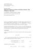
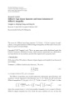
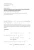
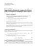
4 EURASIP Journal on Advances in Signal Processing 50 0 0 30 45 −5 −5 25 40 −10 Frequency oﬀset (kHz) −10 35 20 −15 −15 Range (km) 30 −20 15 −20 25 −25 20 −25 10 −30 15 −30 5 10 −35 −35 5 −40 0 −80 −60 −40 −20 0 20 40 60 80 (dB) −40 0 −80 −60 −40 −20 0 20 40 60 80 (dB) Angle (deg) Angle (deg) Figure 3: The beam direction varies as a function of frequency oﬀset. Figure 2: The beam direction varies as a function of range. 0 in the MIMO-FD context, the apparent angle of the trans- mittingbeam GT (r , θ ) is not necessarily equal to that of the −5 receiving beam GR (θ ) at certain ranges. If the transmitting −10 beam is desired to be directed to a known target at (r , θ ), the frequency oﬀset must be deliberately selected to keep the −15 Response (dB) direction consistent with that of the receiving beam. −20 3.2. Frequency Oﬀset-Dependent Beam. Let θ denote the −25 apparent angle of the transmitting beam. Then, the relation- ship between the apparent angle and the nominal angle can −30 be written as [22, 23] −35 Δ f · 2r Δ f · sin θ θ = arcsin sin θ − . + (11) −40 f0 · L f0 0 5 10 15 20 25 30 Frequency oﬀset (kHz) It should be noted that 2r in (11) indicates the round-trip distance, which is diﬀerent from that in [22, 23]. Assume Figure 4: The beam directs to a target at (50 km, 00 ) with diﬀerent the nominal angle θ = 0 and the antenna spacing L = λ0 / 2. frequency oﬀsets. Then, the apparent angle can be written as 4r Δ f θ = arcsin oﬀsets is shown in Figure 4. The beam is repeatedly directed . (12) c to the target with some certain frequency oﬀsets, which can provide additional freedom to choose the frequency oﬀset. The above equation demonstrates that for a known An analytic expression of the frequency oﬀset-dependent nominal angle, if Δ f is ﬁxed, the beam direction is a function beam directed to the target at (r , θ ) can be derived. According of range r . Such beams are called range-dependent beams. to (11), letting the apparent angle equal the nominal angle However, if range r is ﬁxed, the beam direction is a function with π ambiguity, we obtain of Δ f . Such beams can be deﬁned as frequency oﬀset- dependent beams. Δ f 2r Δ f sin θ = nπ + sin θ − n = 0, 1, . . . . sin θ , + f0 L f0 3.3. Examples of Frequency Oﬀset-Dependent Beam. The (13) range dependence is ﬁrst examined for a 10-element standard ULA with Δ f = 30 kHz and f0 = 10 GHz. Figure 2 depicts Then the frequency oﬀset is that the beam varies in the range dimension. Note that there exists π ambiguity, and the beam is directed at angle 00 only f0 at certain ranges. Δ f = nπ n = 0, 1, . . . . , (14) 2r/L − sin θ The frequency oﬀset-dependent beam for a target at range r = 50 km is depicted in Figure 3. The beam direction varies with frequency oﬀset from 0 to 30 kHz. A 1-D cut 3.4. Orthogonal Waveforms. To separate M radiated wave- of the beam directed at (50 km, 00 ) with diﬀerent frequency forms at the receiving end or minimize the interference
EURASIP Journal on Advances in Signal Processing 5 0 0 −10 −10 Magnitude response (dB) Magnitude response (dB) −20 −20 −30 −40 −30 −50 −40 −60 −70 −50 −80 −60 −40 −30 −20 −10 −40 −30 −20 −10 0 10 20 30 40 0 10 20 30 40 Angle (deg) Angle (deg) Subarray Subarray MIMO MIMO MIMO-FD MIMO-FD Figure 5: Beam pattern for MIMO and MIMO-FD arrays with half Figure 6: Beam pattern for MIMO and MIMO-FD arrays with the sparse distance L = 20λ0 / 2. a wavelength spacing. oﬀset Δ f should be a multiple of the least common multiple between waveforms, the correlation of two waveforms must satisfy (LCM) of (14), (17), that is, ⎧ ⎨δ (t ), i = m, π f0 1 Δ f = n · LCM n = 1, 2, . . . . , , (18) si (t ) ∗ sH (t ) = ⎩ (15) 2r/L − sin θ T m i = m, 0, / For comparison, consider a standard ULA with 10 where ∗ denotes the convolution operator. elements. Suppose that the operating frequency is 10 GHz, If the waveform duration is T , the cross-correlation of and the signal duration is T = 1 μs. If the beam is desired two waveforms is to be directed to a target at (35 km, 00 ), the set of Δ f can be selected as T/ 2 si (t )s† (t )dt m −T/ 2 Δ f ≈ n · 67 MHz, n = 1, 2, . . . , (19) T/ 2 1 = exp j 2π f0 + (i − 1)Δ f t according to (18). (16) T −T/ 2 Figure 5 shows the transmit-receive BPs for the MIMO and the MIMO-FD cases, where the frequency oﬀset is × exp − j 2π f0 + (m − 1)Δ f t d t Δ f = 134 MHz. Compared with the phased-array radar, the √ = sinc π (i − m)Δ f · T , MIMO array decreases the beamwidth by a factor of 2 [7]. The peak sidelobe level (PSL) of the MIMO array is about where (†) is the complex conjugate operator. So, to make −26.4 dB, almost twice that of the phased array. The PSL waveforms orthogonal to each other, Δ f should satisfy drops even further to nearly −30 dB for the MIMO-FD array. This demonstrates the eﬀect of the frequency diversity in n Δf = n = 1, 2, . . . . , (17) sidelobe reduction. T The waveforms can coexist if the frequency oﬀset is n/T 4. Simulation Results between two subarray waveforms, that is, the orthogonality of waveforms can be achieved by separating the frequencies In this section, the method to suppress grating lobes of waveforms by an integer multiple of the reciprocal of the based on frequency diversity in coherent MIMO radar with waveform pulse duration. separated subarrays addressed in Section 3 is evaluated by simulation. There are 10 subarrays, and each subarray is 3.5. Selection of Frequency Oﬀset. The frequency oﬀset of a 10-element ULA. The operating frequency is 10 GHz. The duration of each waveform pulse is 1 μs, the target is a MIMO-FD array should satisfy not only (14) to control located at (35 km, 00 ). We change the sparse distance and the the transmitting beam direction, but also (17) to make the frequency oﬀset to test the suppression eﬀect. transmitted waveforms orthogonal. Therefore, the frequency
6 EURASIP Journal on Advances in Signal Processing 0 0 −10 −10 Magnitude response (dB) Magnitude response (dB) −20 −20 −30 −30 −40 −40 −50 −50 −60 −60 −70 −70 −80 −80 −40 −30 −20 −10 −40 −30 −20 −10 0 10 20 30 40 0 10 20 30 40 Angle (deg) Angle (deg) Figure 7: Grating lobes cancelled by the nulls of the subarray beam Subarray with M = 10 and L = 20λ0 / 2. MIMO MIMO-FD Figure 9: Beam pattern for MIMO and MIMO-FD arrays with the sparse distance L = 100λ0 / 2. 0 −10 −16 −18 −20 Magnitude response (dB) −20 −30 Peak sidelobe level (dB) −22 −40 −24 −50 −26 −60 −28 −70 −30 −32 −80 −34 −40 −30 −20 −10 0 10 20 30 40 10 20 30 40 50 60 70 80 90 100 Angle (deg) Sparse distance normalised to wavelength Frequency oﬀset = Subarray MIMO 201 MHz 67 MHz MIMO-FD 134 MHz 268 MHz Figure 8: Beam pattern for MIMO and MIMO-FD arrays with the Figure 10: The PSL versus diﬀerent sparse distances and frequency sparse distance L = 10λ0 / 2. oﬀsets. In fact, for an ULA with the sparse distance L = 20 · First suppose that the sparse distance between subarrays is L = 20 · (λ0 / 2). As described in Section 3, the frequency (λ0 / 2), there exist twelve grating lobes within the angle oﬀset can be set as Δ f = 134 MHz. Figure 6 depicts the interval [−400 , 400 ]. However, only six remain in either the transmit-receive BP. It can be seen that there exist high MIMO or the MIMO-FD BP (see Figure 6). The reason is grating lobes in the MIMO BP. However, the PSL is reduced that the null locations of the subarray beam are just the same to nearly −28.5 dB with frequency diverse waveforms trans- as some certain locations of grating lobes. This is shown in mitted. It should be noted that the subarray beam has two Figure 7. If the number of the nulls in the subarray beam is important eﬀects on the transmit-receive BP. The ﬁrst is that just equal to the number of grating lobes, the grating lobes it functions as an amplitude ﬁlter. The envelope of the MIMO can be totally cancelled out in whether the MIMO or the BP is just the same as the subarray beam. The second is to MIMO-FD BP. In this case, the element number of each cancel out some certain grating lobes using its nulls. subarray is equal to the sparse distance normalized to half a
EURASIP Journal on Advances in Signal Processing 7 10 10 Magnitude response (dB) Magnitude response (dB) 5 5 0 0 −5 −5 −10 −10 −15 −15 −20 −20 −7 −6.5 −6 −5.5 −5 −4.5 −4 −3.5 −3 −2.5 −2 −7 −6.5 −6 −5.5 −5 −4.5 −4 −3.5 −3 −2.5 −2 Angle (deg) Angle (deg) The grating lobes for f9 The grating lobes for f9 The grating lobes for f10 The grating lobes for f10 The ﬁrst grating lobe for f1 The ﬁrst grating lobe for f1 Figure 12: The diﬀerent locations of grating lobes before combin- Figure 11: The diﬀerent locations of grating lobes before combin- ing, Δ f = 268 MHz, L = 20λ0 / 2. ing, Δ f = 201 MHz, L = 20λ0 / 2. oﬀset. However, the suppression eﬀect gets worse for Δ f = wavelength. So, we set the sparse distance as L = 10 · (λ0 / 2), 268 MHz than for Δ f = 201 MHz. This is interpreted in and the cancellation result is demonstrated in Figure 8. The Figures 11, 12, which depict the beams formed at diﬀerent PSL for the MIMO BP is −26.4 dB, and it is the same as that of a ﬁlled MIMO array. Note that a lower PSL for MIMO-FD frequencies before the coherent combining. It can be seen BP (nearly −31 dB) is achieved. that with Δ f = 201 MHz, the 2nd grating lobe for the We further test the suppression eﬀect for an even larger frequency f10 is near in the 3-dB beamwidth of the 1st sparse distance L = 100(λ0 / 2). The result is depicted in grating lobe for the frequency f1 . However, when Δ f is Figure 9. The suppression eﬀect is degraded with the PSL larger than 268 MHz, the 2nd grating lobe for the frequency improved to −21 dB. The reason is that the receiving beams f9 moves into the 3-dB beamwidth of the 1st grating lobe formed at diﬀerent frequencies exhibit similar properties for the frequency f1 . Since the grating lobes are mixed, the suppression eﬀect will surely get worse. only in the region of mainlobe and neighboring sidelobes. Furthermore, for a ﬁxed subarray number and a ﬁxed subarray size, the larger the sparse distance is, the more 5. Conclusion the number of grating lobes in the beam is. With more neighboring grating lobes exhibiting similar properties, the A method based on frequency diversity to suppress grating suppression eﬀect surely becomes worse. lobes in sparse MIMO aperture radar is proposed in this It is evident that a larger frequency oﬀset is helpful paper. By the frequency diversity across the transmitting in suppressing grating lobes. Though the receiving beams array, the locations of grating lobes in the receiving beams formed at diﬀerent frequencies exhibit similar properties in are totally changed. Coherently combining the M receiving the mainlobe region, the locations of grating lobes become beams formed at diﬀerent frequencies can suppress grating progressively diﬀerent with the frequency oﬀset increasing. lobes to a low level. The resultant transmit-receive BP is When all the M receiving beams are combined, the portion of composed of the range-dependent transmitting beam and the mainlobe region remains unchanged, and in the sidelobe the combined receiving beam. We demonstrate that, even region, the peaks will reduce to a lower level for a larger though the transmitting beam is range-dependent, the beam Δf. can be precisely steered to a given target by deliberately There exists an upper limit to the frequency oﬀset Δ f to selecting a set of Δ f . The simulation results show that with achieve the optimum suppression eﬀect. For the movement a properly selected frequency oﬀset, the method is eﬀective of the nth grating lobe by angle Δθ , the transmit wavelength in suppressing grating lobes in sparse MIMO aperture should be changed by Δλ with Δθ = sin−1 (nλ0 /L) − radars. sin−1 (nλi /L) ≈ nΔλ/L. If the (n + 1)th grating lobe for the wavelength λi moves into the 3-dB beamwidth of the nth grating lobe for the wavelength λ1 , some additional Appendix energy will remain in this location. Thus, the suppression eﬀect will be degraded. In Figure 10, we compare the A. Deriving the Transmit-Receive BP of suppression eﬀects for diﬀerent Δ f with the given simu- MIMO-FD Array lation parameters. The sparse distance is changed in the Let φ = (4πr/c), and let ϕ = −(2π/c)L sin θ , then the interval [20(λ0 / 2), 200(λ0 / 2)]. Evidently, a better grating lobe suppression eﬀect can be achieved using a larger frequency MIMO-FD array response can be rewritten as
8 EURASIP Journal on Advances in Signal Processing ⎛ ⎞ · · · asub f1 , θ A asub f1 , θ exp j f1 φ asub f1 , θ exp j f1 ϕ + φ ⎜ ⎟ ⎜ · · · asub f2 , θ B ⎟ asub f2 , θ exp j f2 ϕ + φ asub f2 , θ exp j f2 2ϕ + φ B(θ ) = ⎜ ⎟ ⎜ ⎟ (A.1) ⎜ ⎟, . . . ⎜ ⎟ . . . ⎜ ⎟ ··· . . . ⎝ ⎠ · · · asub fM , θ C asub fM , θ exp j fM (M − 1)ϕ + φ asub fM , θ exp j fM M ϕ + φ = B1 (θ ) B2 (θ ), A = exp j f1 (M − 1)ϕ + φ , B = exp j f2 M ϕ + φ , C = exp j fM 2(M − 1)ϕ + φ , (A.2) where represents the Hadamard product, and ⎡ ⎤ ··· exp j f1 φ exp j f1 φ exp j f1 φ ⎢ ⎥ ⎢ ⎥ ··· exp j f2 ϕ + φ exp j f2 ϕ + φ exp j f2 ϕ + φ ⎢ ⎥ ⎢ ⎥ B1 (θ ) = ⎢ ⎥, . . . ⎢ ⎥ . . . ⎢ ⎥ ··· . . . ⎣ ⎦ exp j fM (M − 1)ϕ + φ exp j fM (M − 1)ϕ + φ · · · exp j fM (M − 1)ϕ + φ (A.3) ⎡ ⎤ asub f1 , θ · 1 asub f1 , θ · exp j f1 ϕ ··· asub f1 , θ · exp j f1 (M − 1)ϕ ⎢ ⎥ ⎢a asub f2 , θ · exp j f2 (M − 1)ϕ ⎥ ⎢ sub f2 , θ · 1 asub f2 , θ · exp j f2 ϕ ··· ⎥ ⎢ ⎥ B2 (θ ) = ⎢ ⎥. . . . ⎢ ⎥ . . . ⎢ ⎥ ··· . . . ⎣ ⎦ asub fM , θ · 1 asub fM , θ · exp j fM ϕ · · · asub fM , θ · exp j fM (M − 1)ϕ It is worthwhile to notice that B1 (θ ) can be viewed as the The matched weight vector of the beamformer can be aMIMO-FD (θ0 ) = b(r , θ0 ) ⊗ IM ×1 a( f , θ0 ), and the resultant transmitting array response. B2 (θ ) represents the receiving array response with diﬀerent frequencies transmitted from transmit-receive BP is the same subarray. By joining the matrix B(θ ) into an MM ×1 vector, the MIMO-FD array response vector can be written as 2 H GMIMO-FD (θ ) = aMIMO-FD (θ0 )aMIMO-FD (θ ) 2 H = (b(r , θ0 ) ⊗ IM ×1 ) (b(r , θ ) ⊗ IM ×1 ) aMIMO-FD (θ ) = b(r , θ ) ⊗ IM ×1 a f ,θ , (A.4) 2 × aH f , θ0 a f , θ 2 where IM ×1 is an M × 1 length identity vector, and = bH (r , θ0 )b(r , θ ) 2 M 1 aH fi , θ0 a fi , θ × M i=1 b(r , θ ) = exp j f1 φ , exp j f2 ϕ + φ , . . . , = GT (r , θ )GR (θ ), T exp j fM (M − 1)ϕ + φ , (A.5) (A.7) T a f , θ = a f1 , θ , . . . , a fi , θ , . . . , a fM , θ , where with 2 GT (r , θ ) = bH (r , θ0 )b(r , θ ) , (A.8) 2 M a fi , θ = asub fi , θ ⊗ 1, exp j fi ϕ , . . . , exp j fi (M − 1)ϕ . 1 aH fi , θ0 a fi , θ GR (θ ) = . (A.6) M i=1
EURASIP Journal on Advances in Signal Processing 9 B. The Relationship between PSL/ASL and Δ f where E{·} is the expected value of {·}. For a sparse array M L/λi and a high fi Δ f , the second term is much Since the grating lobe suppression eﬀect is achieved by coher- smaller than the ﬁrst one in the sidelobe region. Then ently combining the M receiving beams formed at diﬀerent frequencies, the impact of subarray beam is omitted here. sin Δ f ϕ − ϕ0 / 2 Ri,i+1 ∼ M = . (B.3) Though the beams formed at diﬀerent frequencies exhibit Δ f ϕ − ϕ0 / 2 similar properties in the mainlobe region, the correlation in the remainder part progressively decreases. The manner The two beams are decorrelated in the sidelobe region when Δ f (ϕ − ϕ0 )/ 2 = π . And so in which the region of sidelobes decorrelates with frequency can be calculated from the cross correlation function of two beams formed at two diﬀerent frequencies [20]. 2π c Δf = = ϕ − ϕ0 (M − 1)L(sin θ − sin θ0 ) Each receiving beam can be written as (B.4) λ0 f0 = . M (M − 1)L(sin θ − sin θ0 ) 2π Fi (θ ) = exp − j fi L(m − 1 )(sin θ − sin θ0 ) c m=1 In addition, the ratio of the Peak Sidelobe Level (PSL) to (B.1) the Average Sidelobe Level (ASL) of a linear random sparse M = exp j fi (m − 1) ϕ − ϕ0 , array is approximately [16] m=1 S(1 + |sin θ0 |) PSL/ ASL ∼ ln = , (B.5) λ0 where ϕ0 = −(2π/c)L sin θ0 . The cross-correlation function of the two receiving beams formed at two subsequent where S is the array aperture length. If the sparse array frequencies is is uniformly distributed, S = (M − 1)L. In this case, the PSL/ASL is Ri,i+1 = E Fi (θ )Fi† (θ ) (M − 1)L(1 + |sin θ0 |) +1 PSL/ ASL ∼ ln = . (B.6) ⎧ λ0 ⎨ M =E exp j fi (m − 1) ϕ − ϕ0 ⎩ Combining (B.4) and (B.6) we can obtain m=1 ⎫ 1 + |sin θ0 | f0 PSL ∼ ⎬ M · = ln . (B.7) × exp − j fi+1 (n − 1) ϕ − ϕ0 ⎭ Δ f sin θ − sin θ0 ASL n=1 Variation of the frequency oﬀset Δ f does not alter the ASL. M M Hence, the PSL can be reduced to get closer to the ASL with = E exp j fi (m − 1) ϕ − ϕ0 a larger Δ f . m=1 n=1 × exp − j fi+1 (n − 1) ϕ − ϕ0 References ⎧ ⎫ ⎪ ⎪ ⎪ ⎪ ⎨ ⎬ M [1] E. Fishler, A. Haimovich, R. Blum, D. Chizhik, L. Cimini, and =E exp − j Δ f (m − 1) ϕ − ϕ0 ⎪ R. Valenzuela, “MIMO radar: an idea whose time has come,” ⎪ ⎪m=1 ⎪ ⎩ ⎭ in Proceedings of the IEEE National Radar Conference, pp. 71– (B.2) n=m 78, Philadelphia, Pa, USA, April 2004. ⎧ ⎫ ⎨ ⎬ M [2] E. Fishler, A. Haimovich, R. Blum, L. Cimini, D. Chizhik, and exp j fi (m − 1) ϕ − ϕ0 ⎭ + E⎩ R. Valenzuela, “Performance of MIMO radar systems: advan- m=1 tages of angular diversity,” in Proceedings of the 38th Asilomar ⎧ ⎫ Conference on Signals, Systems and Computers (ACSSC ’04), ⎪ ⎪ ⎪ ⎪ ⎨ ⎬ vol. 1, pp. 305–309, Paciﬁc Grove, Calif, USA, November 2004. M ×E exp − j fi+1 (n − 1) ϕ − ϕ0 ⎪ [3] E. Fishler, A. Haimovich, R. S. Blum, L. Cimini Jr., D. ⎪ ⎪ n=1 ⎪ ⎩ ⎭ Chizhik, and R. A. Valenzuela, “Spatial diversity in radars- n=m / models and detection performance,” IEEE Transactions on Signal Processing, vol. 54, no. 3, pp. 823–838, 2006. sin Δ f ϕ − ϕ0 / 2 =M [4] V. F. Mecca, D. Ramakrishnan, and J. L. Krolik, “MIMO Δ f ϕ − ϕ0 / 2 radar space-time adaptive processing for multipath clutter mitigation,” in Proceedings of the 4th IEEE Sensor Array and sin fi ϕ − ϕ0 / 2 + M (M − 1) Multichannel Signal Processing Workshop (SAM ’06), pp. 249– fi ϕ − ϕ0 / 2 253, Waltham, Mass, USA, July 2006. [5] P. Stoica, J. Li, and Y. Xie, “On probing signal design for MIMO sin fi+1 ϕ − ϕ0 / 2 · radar,” IEEE Transactions on Signal Processing, vol. 55, no. 8, , fi+1 ϕ − ϕ0 / 2 pp. 4151–4161, 2007.
10 EURASIP Journal on Advances in Signal Processing [22] P. Antonik, M. C. Wicks, H. D. Griﬃths, and C. J. Baker, [6] D. W. Bliss and K. W. Forsythe, “Multiple-input multiple- output (MIMO) radar and imaging: degrees of freedom and “Frequency diverse array radars,” in Proceedings of the IEEE resolution,” in Proceedings of the 37th Asilomar Conference on Radar Conference, pp. 215–217, Verona, NY, USA, April 2006. [23] P. Antonik, M. C. Wicks, H. D. Griﬃths, and C. J. Baker, Signals, Systems and Computers (ACSSC ’03), vol. 1, pp. 54–59, Paciﬁc Grove, Calif, USA, November 2003. “Range dependent beamforming using element level wave- [7] I. Bekkerman and J. Tabrikian, “Target detection and local- form diversity,” in Proceedings of the International Waveform ization using MIMO radars and sonars,” IEEE Transactions on Diversity and Design Conference, Lihue, Hawaii, USA, January Signal Processing, vol. 54, no. 10, pp. 3873–3883, 2006. 2006. [8] F. C. Robey, S. Coutts, D. Weikle, J. C. McHarg, and K. [24] P. Baizert, T. B. Hale, M. A. Temple, and M. C. Wicks, Cuomo, “MIMO radar theory and experimental results,” in “Forward-looking radar GMTI beneﬁts using a linear fre- Proceedings of the 38th Asilomar Conference on Signals, Systems quency diverse array,” Electronics Letters, vol. 42, no. 22, pp. and Computers (ACSSC ’04), vol. 1, pp. 300–304, Paciﬁc Grove, 1311–1312, 2006. Calif, USA, November 2004. [9] J. Li, P. Stoica, L. Xu, and W. Roberts, “On parameter identiﬁability of MIMO radar,” IEEE Signal Processing Letters, vol. 14, no. 12, pp. 968–971, 2007. [10] H. Yan, J. Li, and G. Liao, “Multitarget identiﬁcation and localization using bistatic MIMO radar systems,” EURASIP Journal on Advances in Signal Processing, vol. 2008, Article ID 283483, 8 pages, 2008. [11] D. R. Fuhrmann and G. S. Antonio, “Transmit beamforming for MIMO radar systems using partial signal correlation,” in Proceedings of the 38th Asilomar Conference on Signals, Systems and Computers (ACSSC ’04), vol. 1, pp. 295–299, Paciﬁc Grove, Calif, USA, November 2004. [12] L. Xu and J. Li, “Iterative generalized-likelihood ratio test for MIMO radar,” IEEE Transactions on Signal Processing, vol. 55, no. 6, pp. 2375–2385, 2007. [13] J. Li and P. Stoica, “MIMO radar with colocated antennas,” IEEE Signal Processing Magazine, vol. 24, no. 5, pp. 106–114, 2007. [14] N. H. Lehmann, A. M. Haimovich, R. S. Blum, and L. Cimini, “High resolution capabilities of MIMO radar,” in Proceedings of the 40th Asilomar Conference on Signals, Systems and Computers (ACSSC ’06), pp. 25–30, Paciﬁc Grove, Calif, USA, November 2006. [15] A. M. Haimovich, R. S. Blum, and L. Cimini, “MIMO radar with widely separated antennas,” IEEE Signal Processing Magazine, vol. 25, no. 1, pp. 116–129, 2008. [16] B. D. Steinberg, “The peak sidelobe of the phased array having randomly located elements,” IEEE Transaction on Antenna and Propagation, vol. 20, no. 2, pp. 129–137, 1972. [17] M. G. Bray, D. H. Werner, D. W. Boeringer, and D. W. Machuga, “Optimization of thinned aperiodic linear phased arrays using genetic algorithms to reduce grating lobes during scanning,” IEEE Transactions on Antennas and Propagation, vol. 50, no. 12, pp. 1732–1742, 2002. [18] M. A. Haleem and A. M. Haimovich, “On the distribution of ambiguity levels in MIMO radar,” in Proceedings of the 42nd Asilomar Conference on Signals, Systems and Computers (ACSSC ’08), Paciﬁc Grove, Calif, USA, November 2008. [19] M. Skolnik, “Resolution of angular ambiguities in radar array antennas with widely-spaced elements and grating lobes,” IEEE Transaction on Antenna and Propagation, vol. 10, no. 3, pp. 351–352, 1962. [20] B. D. Steinberg and E. H. Attia, “Sidelobe reduction of random arrays by element position and frequency diversity,” IEEE Transactions on Antennas and Propagation, vol. 31, no. 6, pp. 922–930, 1983. [21] D. R. Kirk, J. S. Bergin, P. M. Techau, and J. E. Don Carlos, “Multi-static coherent sparse aperture approach to precision target detection and engagement,” in Proceedings of the IEEE Radar Conference, pp. 579–584, Arlington, Va, USA, May 2005.

CÓ THỂ BẠN MUỐN DOWNLOAD

LV.09: Bộ Luận Văn Tốt Nghiệp Chuyên Ngành Quản Trị Kinh Doanh

81 tài liệu

1637 lượt tải

ERROR:connection to 10.20.1.100:9315 failed (errno=111, msg=Connection refused)
ERROR:connection to 10.20.1.100:9315 failed (errno=111, msg=Connection refused)

THÔNG TIN

TRỢ GIÚP

HỖ TRỢ KHÁCH HÀNG

Theo dõi chúng tôi

Chịu trách nhiệm nội dung:

Nguyễn Công Hà - Giám đốc Công ty TNHH TÀI LIỆU TRỰC TUYẾN VI NA

LIÊN HỆ

Địa chỉ: P402, 54A Nơ Trang Long, Phường 14, Q.Bình Thạnh, TP.HCM

Hotline: 093 303 0098

Email: support@tailieu.vn