Báo cáo hóa học: " Research Article Computationally Efﬁcient DOA and Polarization Estimation of Coherent Sources with Linear Electromagnetic Vector-Sensor Array"

Chia sẻ: Nguyen Minh Thang | Ngày: | Loại File: PDF | Số trang:10

Thêm vào BST

Báo xấu

38
lượt xem 5
download

Download Vui lòng tải xuống để xem tài liệu đầy đủ

Tuyển tập báo cáo các nghiên cứu khoa học quốc tế ngành hóa học dành cho các bạn yêu hóa học tham khảo đề tài: Research Article Computationally Efﬁcient DOA and Polarization Estimation of Coherent Sources with Linear Electromagnetic Vector-Sensor Array

Chủ đề:

Bình luận(0) Đăng nhập để gửi bình luận!

Lưu

Nội dung Text: Báo cáo hóa học: " Research Article Computationally Efﬁcient DOA and Polarization Estimation of Coherent Sources with Linear Electromagnetic Vector-Sensor Array"

Hindawi Publishing Corporation EURASIP Journal on Advances in Signal Processing Volume 2011, Article ID 490289, 10 pages doi:10.1155/2011/490289 Research Article Computationally Efﬁcient DOA and Polarization Estimation of Coherent Sources with Linear Electromagnetic Vector-Sensor Array Zhaoting Liu,1 Jing He,2 and Zhong Liu1 1 Department of Electronic Engineering, Nanjing University of Science and Technology, Nanjing, Jiangsu 210094, China 2 Department of Electrical and Computer Engineering, Concordia University, Montreal, QC, Canada H3G 2W1 Correspondence should be addressed to Zhaoting Liu, liuzhaoting@163.com Received 3 September 2010; Revised 10 December 2010; Accepted 16 January 2011 Academic Editor: Ana P´ rez-Neira e Copyright © 2011 Zhaoting Liu et al. This is an open access article distributed under the Creative Commons Attribution License, which permits unrestricted use, distribution, and reproduction in any medium, provided the original work is properly cited. This paper studies the problem of direction ﬁnding and polarization estimation of coherent sources using a uniform linear electromagnetic vector-sensor (EmVS) array. A novel preprocessing algorithm based on EmVS subarray averaging (EVSA) is ﬁrstly proposed to decorrelate sources’ coherency. Then, the proposed EVSA algorithm is combined with the propagator method (PM) to estimate the EmVS steering vector, and thus estimate the direction-of-arrival (DOA) and the polarization parameters by a vector cross-product operation. Compared with the existing estimate methods, the proposed EVSA-PM enables decorrelation of more coherent signals, joint estimation of the DOA and polarization of coherent sources with a lower computational complexity, and requires no limitation of the intervector sensor spacing within a half-wavelength to guarantee unique and unambiguous angle estimates. Also, the EVSA-PM can estimate these parameters by parameter-space searching techniques. Monte-Carlo simulations are presented to verify the eﬃcacy of the proposed algorithm. 1. Introduction investigations [10–12, 16–19]. The signal subspace and noise subspace are usually constructed by decomposing A typical electromagnetic vector-sensor (EmVS) consists the column space of the data correlation matrix with of six component sensors conﬁgured by two orthogonal the eigen-decomposition (or singular value decomposition) triads of dipole and loop antennas with the same phase techniques [22, 23]. Because the decomposing process is center. Therefore, an EmVS can simultaneously measure computationally intensive and time consuming, the eigen- the three components of the electric ﬁeld and the three structure-based techniques may be unsuitable for many components of the magnetic ﬁeld. Since its introduction into practical situations, especially when the number of vector signal processing community [1, 2], a signiﬁcant number sensors is large and/or the directions of impinging sources of research has been done on EmVS array processing should be tracked in an online manner. [3–19]. For application considerations, diﬀerent types of Furthermore, the eigenstructure-based direction ﬁnding EmVS containing part of the six sensors are devised and techniques using the EmVS arrays usually assume incoherent manufactured [3, 20, 21]. signals, that is, that the signal covariance matrix has full rank. In the study of direction ﬁnding applications, conven- This assumption is often violated in scenarios where multi- tional eigenstructure-based source localization techniques path exists. Coherent signals could reduce the rank of signal have been extended to the case of the EmVS array. ESPRIT/ covariance matrix below the number of incident signals, MUSIC algorithms using EmVS arrays obtain thorough and hence, degrade critically the algorithmic performance.
2 EURASIP Journal on Advances in Signal Processing To deal with the coherent signals using the EmVS array, a the kth unit-power electromagnetic source signal produces the following 6 × 1 vector: polarization smoothing algorithm (PSA) has been proposed to restore the rank of signal subspace [19]. The PSA does not reduce the eﬀective array aperture length and has no limit to c θk , ϕk , γk , ηk array geometries. However, the PSA-based method has non- ⎡ ⎤ ⎡ ⎤ c1,k ex,k negligible drawbacks. (1) It assumes the intervector sensor ⎢⎥ ⎢ ⎥ ⎢c2,k ⎥ ⎢ e y ,k ⎥ spacing within a half-wavelength to guarantee unique and ⎢⎥ ⎢ ⎥ ⎢⎥ ⎢ ⎥ unambiguous angle estimates; (2) it is not able to estimate ⎢⎥ ⎢e ⎥ def ⎢c3,k ⎥ def ⎢ z ,k ⎥ =⎢ ⎥= ⎢ ⎥ the polarization of impinging electromagnetic waves; (3) ⎢⎥ ⎢ ⎥ ⎢c4,k ⎥ ⎢hx,k ⎥ the EmVS type limits the maximum number of resolvable ⎢⎥ ⎢ ⎥ ⎢⎥ ⎢ ⎥ coherent signals. ⎢c5,k ⎥ ⎢ h y ,k ⎥ ⎣⎦ ⎣ ⎦ In this paper, we employ a uniform linear EmVS c6,k hz,k array to perform parameter estimation of coherent sources. (1) ⎡ ⎤ Firstly, to decorrelate the coherent sources, an EmVS sub- − sin ϕk cos ϕk cos θk ⎢ ⎥ array averaging-based pre-processing (EVSA) algorithm is ⎢ sin ϕk cos θk ⎥ cos ϕk ⎢ ⎥ developed. Then the EVSA algorithm is coupled with the ⎢ ⎥⎡ ⎥ sin γ e jηk ⎤ ⎢ − sin θ ⎢ ⎥ 0 propagator method (PM) [24, 25] to estimate parameters k k ⎢ ⎥⎣ ⎦, =⎢ ⎥ of the coherent sources without eigen-decomposition or ⎢ − sin ϕk − cos ϕk cos θk ⎥ cos γk ⎢ ⎥ singular value decomposition unlike the ESPRIT/MUSIC- ⎢ ⎥ ⎢ cos ϕk − sin ϕk cos θk ⎥ def g γ ,η ⎣ ⎦ = ( k k) based methods. By using the vector cross-product of the electric ﬁeld vector estimate and the magnetic ﬁeld vector 0 sin θk estimate, the proposed EVSA-PM can estimate both the def = Θ(θk ,φk ) DOA and polarization parameters, hence, can overcome the drawbacks of the PSA-based algorithms to some extent. The def def vector cross-product estimator is valid to a six-component where ek = [ex,k , e y,k , ez,k ]T and hk = [hx,k , h y,k , hz,k ]T EmVS array. For the array comprising any types of EmVSs, denote the electric ﬁeld vector and the magnetic ﬁeld vector, the EVSA-PM with parameter-space searching techniques respectively. is developed to estimate the parameters. The EVSA-PM The intersensor spatial phase factor for the kth inci- can be regarded as an extension of the subspace-based def dent signal and the mth vector sensor is qm (θk , ϕk ) = method without eigendecomposition (SUMWE) [26] to the def def e j 2π (xm uk + ym vk )/λ , where uk = sin θk cos ϕk and vk = case of the EmVS arrays. The SUMWE is also a PM-based sin θk sin ϕk signify the direction cosines along the x-axis method, which estimates the DOA of coherent sources using and y-axis, respectively. (xm , ym ) is the location of the mth unpolarized scalar sensors by an iterative angle searching. vector sensor, λ equals the signals’ wavelength. Denoting the However, the proposed methods make use of more available spacing between adjacent vector sensors as (Δx , Δ y ), we have electromagnetic information, and hence, should outperform xm = x1 + (m − 1)Δx , ym = y1 + (m − 1)Δ y . The 6 × 1 the SUMWE algorithm in accuracy and resolution of DOA measurement vector corresponding to the mth vector sensor estimation. can be expressed as The rest of this paper is organized as follows. Section 2 formulates the mathematical data model of EmVS array. def T xm (t ) = xm,1 (t ), . . . , xm,6 (t ) Section 3 develops the proposed EmVS-PM. Section 4 presents the simulation results to verify the eﬃcacy of the (2) K EmVS-PM. Section 5 concludes the paper. = qm θk , ϕk c θk , ϕk , γk , ηk sk (t ) + wm (t ), k=1 2. Mathematical Data Model where wm (t ) = [wm,1 (t ), . . . , wm,6 (t )]T is the additive zero- Assume that K narrowband completely polarized coherent mean complex noise and independent to all signals. xm,n (t ) signals impinge upon a uniform linear EmVS array with M and wm,n (t ) refer to the measurement and the noise corre- vector sensors (M > 2K ), and the array is neither mutual sponding to the mth vector sensor’s nth component, respec- coupling nor cross-polarization eﬀects. The K is known tively; sk (t ) represents the kth source’s complex envelope. Without loss of generality, we consider the signals {sk (t )} are in advance and the kth incident source is parameterized {θk , ϕk , γk , ηk }, where 0 ≤ θk ≤ π/ 2 denotes the kth source’s all coherent so that they are all some complex multiples of a elevation angle measured from the vertical z-axis, 0 ≤ ϕk ≤ common signal s1 (t ). Then, under the ﬂat-fading multipath 2π represents the kth source’s azimuth angle, 0 ≤ γk ≤ π/ 2 propagation, they can be expressed as sk (t ) = βk s1 (t ) [26, 27], where βk is the multipath coeﬃcient that represents the refers to the kth source’s auxiliary polarization angle, and −π ≤ ηk ≤ π symbolizes the kth source’s polarization phase complex attenuation of the kth signal with respect to the ﬁrst diﬀerence. For a six-component EmVS, the steering vector of one (β1 = 1 and βk = 0). /
EURASIP Journal on Advances in Signal Processing 3 def β = [β1 , . . . , βK ]T . Similarly, the cross-correlation vector For the entire vector-sensor array, the array manifold, a(θk , ϕk , γk , ηk ) ∈ C 6M ×1 , is given by ϕl,n ∈ C 6K ×1 between zl (t ) and x1,n (t ) is as follows def def a θk , ϕk , γk , ηk = q θk , ϕk ⊗ c θk , ϕk , γk , ηk , ∗ ϕl,n = E zl (t )x1,n (t ) (3) (7) where ⊗ symbolizes the Kronecker product operator, = ρ1,n rs A0 Dl−1 β, l = 2, . . . , L; n = 1, . . . , 6. def q(θk , ϕk ) = [q1 (θk , ϕk ), . . . , qM (θk , ϕk )]T . With a total of K Let us rewrite the vector ϕl,n as a 6 × K matrix signals, the entire 6M × 1 output vector measured by the EmVS array at time t has the complex envelope represented def Φl,n = J1 ϕl,n , . . . , JK ϕl,n as T = ρM ,n rs A1 Dl−1 β, . . . , AK Dl−1 β T T z(t ) = x1 (t ), . . . , xM (t ) (8) = ρM ,n rs Al β, . . . , DK −1 β K (4) = a θk , ϕk , γk , ηk sk (t ) + n(t ) k=1 = ρM ,n rs Al BQT , = As(t ) + n(t ), def def where Jk = [06,6(k−1) , I6 , 06,6(K −k) ]; B = diag(β1 , . . . , βK ); where A ∈ C 6M ×K , s(t ) ∈ C K ×1 , n(t ) ∈ C 6M ×1 , and A = Al is the 6 × K matrix with the column ck ql (θk , ϕk ), k = 1, . . . , 6; Q is the K × K matrix with the column [a(θ1 , ϕ1 , γ1 , η1 ), . . . , a(θK , ϕK , γK , ηK )]; s(t ) = [s1 (t ), . . . , [q1 (θk , ϕk ), . . . , qK (θk , ϕk )]T . Similarly, the vector ϕl,n can be sK (t )]T , n(t ) = [w1 (t ), . . . , wM (t )]T . T T rewritten as 3. Algorithm Development def Φl,n = J1 ϕl,n , . . . , JK ϕl,n = ρ1,n rs Al BQT . (9) This section is devoted to the algorithm development. Therefore, concatenating Φl,n for l = 1, . . ., L − 1 and Φl,n for Section 3.1 develops the EVSA algorithm, Section 3.2 l = 2, . . . , L, respectively, we can get two correlation matrices describes EVSA-PM algorithm for estimating both DOA and polarization parameters from the available EmVS steering T def Rn = ΦT n , ΦT n , . . . , ΦTL−1),n = ρM ,n rs ABQT , vector estimates and Section 3.3 is for parameters estimation ( 1, 2, by parameter-space searching techniques. (10) T T T T def Rn = Φ2,n , Φ3,n , . . . , ΦL,n = ρ1,n rs ABDQT , 3.1. EVSA Algorithm. Let us consider the subarray averaging scheme with a linear EmVS array, which is divided into def where Rn ∈ C 6(L−1)×K , Rn ∈ C 6(L−1)×K , and A = [AT , . . . , 1 L overlapping subarrays with K vector sensors and the lth AT−1 ]T includes the ﬁrst 6(L − 1) rows of A. With (10), the subarray comprises the lth to (l + K − 1)th vector sensor, L where L = M − K + 1. We use the ﬁrst vector sensor as EmVS subarray averaging (EVSA) matrix can be formulated a reference (x1 = 0, y1 = 0), and then the corresponding as 6K × 1 signal vector is given as def R = R1 , . . . , R6 , R1 , . . . , R6 = AΩ, (11) T def l−1 xlT (t ), . . . , xlT K −1 (t ) zl (t ) = = A0 D s(t ) + nl (t ), (5) + def where Ω = rs B[ρM ,1 QT , . . . , ρM ,6 QT , ρ1,1 DQT , . . . , ρ1,6 DQT ]. Note that B and D are diagonal matrices with nonzero def where D ∈ C K ×K , and D = diag(e j 2π (Δx u1 +Δ y v1 )/λ , . . . , diagonal elements, and Q is full rank when all sources e j 2π (Δx uK +Δ y vK )/λ ); A0 ∈ C 6K ×K contains the ﬁrst 6K rows of A; impinge with the distinct incident directions. Then the Rn def nl (t ) = [wlT (t ), . . . , wlT K −1 (t )]T . We can calculate the cross- and Rn are of rank K , and hence, R is of rank K and can be + correlation vector ϕl,n ∈ C 6K ×1 between zl (t ) and xM ,n (t ) used to estimate the DOA and the polarization parameters of the coherent sources. def ∗ ϕl,n = E zl (t )xM ,n (t ) In realistic cases where only a ﬁnite number of snapshots are available, the cross-correlation vector ϕl,n and ϕl,n can = A0 Dl−1 E s(t )sH (t ) a∗ ,n + E nl (t )wM ,n ∗ ∗ S be estimated as ϕl,n = t =1 zl (t )xM ,n (t )/S and ϕl,n = M ∗ S t =1 zl (t )x1,n (t )/S, where S denotes the number of snapshots. = ρM ,n rs A0 Dl−1 β, l = 1, . . . , L − 1; n = 1, . . . , 6, With ϕl,n and ϕl,n , the matrix R is accordingly obtained using (6) (8)–(11). Note that the proposed EVSA algorithm can also be used def where E{·} denotes the expectation, rs = E{s1 (t )s∗ (t )}, 1 to the case of partly coherent or incoherent signals. To see def def ρl,n = βH a∗n , al,n = [ql (θ1 , ϕ1 )cn,1 , . . .,ql (θK , ϕK )cn,K ]T , this, we assume that the ﬁrst K1 (1 ≤ K1 ≤ K ) incident l,
4 EURASIP Journal on Advances in Signal Processing where ei is the 6(L − 1) dimensional unit vector whose ith signals are coherent and the others are uncorrelated with these signals and with each other. Then after some algebraic element is 1 and other elements are zero. In addition, we manipulations, we can obtain deﬁne def Re = ET R = Ae Ω, (14) Rn = ρM ,n rs1 ABQT + ARAH ,n QT , M (12) Rn = ρ1,n rs1 ABDQT + ADRAHn QT , T def Ae = ET A = AT , . . . , AT 1, , (15) e,1 e,6 where Ae ∈ C 6(L−1)×K , Ae,n ∈ C (L−1)×K (n = 1, . . . , 6) H def def def where ρl,n = β a∗n , β = [β1 , . . . , βK1 , 0, . . . , 0]T , B = l, is a submatrix whose kth column is given as qe (θk , ϕk )cn,k def def diag(β1 , . . . , βK1 , 0, . . . , 0), rsk = E{sk (t )s∗ (t )}, R = diag(0, def with qe (θk , ϕk ) = [q1 (θk , ϕk ), . . . , qL−1 (θk , ϕk )]T . These k def . . . , rsK1 +1 , . . . , rsK ), Al,n = diag(ql (θ1 , ϕ1 )cn,1 , . . . , ql (θK , submatrices are related with each other by ϕK )cn,K ). It is easy to ﬁnd that the rank of Rn and Rn still Ae,n = Ae,1 Λn , (16) equals K when all sources impinge with the distinct incident directions. def def where Λn ∈ C K ×K and Λn = diag(dn,1 , . . . , dn,K ) with dn,k = Remarks. (1) The proposed EVSA algorithm is still eﬀective cn,k /c1,k denoting the kth source’s invariant factor between in the case of partly coherent or incoherent sources in the ﬁrst and the nth EmVS component. which there exist two incoherent sources with the same We can divide Ae,n into incident directions but with the distinct polarizations. As ⎡ ⎤ shown in the appendix, the matrix R deﬁned in (11) has full A(1) e,n Ae,n = ⎣ ⎦, n = 1, . . . , 6, rank. However, neither the PSA [19] nor the SUMWE [26] (17) (2) Ae,n algorithm can be so. (2) The EVSA algorithm needs low computations. As (1) (2) where Ae,n ∈ C K ×K and Ae,n ∈ C (L−1−K )×K . Therefore, Ae,n seen from (6) and (7), the EVSA only needs compute the cross-correlations, which require 72(L − 1) cross-correlation can be rewritten as ⎡ ⎤ operations. However, most of EmVS direction ﬁnding algo- A(1) rithms require to compute the correlations of all array data Ae = ⎣ ⎦, e,1 (18) with (6M )2 correlation operations. U (3) The EVSA-based method may estimate both DOA def (2) (1) (2) (1) (2) where U = [(Ae,1 )T , (Ae,2 )T , (Ae,2 )T , . . . , (Ae,6 )T , (Ae,6 )T ]T . and polarization parameters, while the PSA-based one can only estimate the DOA parameters because of the polariza- Obviously, A(1) is a matrix with full rank. The K × (6L − 6 − e,n tion smoothing. K ) propagator matrix P can be deﬁned as a unique linear (4) From (11), the EVSA algorithm can decorrelate more operator which relates the matrices A(1) and U through the e,1 coherent sources than the PSA can do. The EVSA algorithm equation can decorrelate up-to L − 2 coherent sources regardless of EmVS’s types, while the PSA can only decorrelate 6 PH A(1) = U. (19) e,1 coherent sources for six-component EmVS array, 4 for quadrature polarized array [19] and 2 for dual polarized We partition PH into PH = [PT , PT , . . . , PT ]T , where P1 to 1 2 11 array [19]. By coupling the forward/backward (FB) averaging P11 have the dimensions identical to A(2) , A(1) , A(2) , A(1) , A(2) , technique [27], the maximum number of the coherent e,1 e,2 e,2 e,3 e,3 (1) (2) (1) (2) (1) (2) Ae,4 ,Ae,4 , Ae,5 , Ae,5 , Ae,6 , and Ae,6 , respectively. Thus, we have signals decorrelated by the PSA is doubled, however, it is only valid for the case of the symmetric array, for instance, (1) (2) P1 Ae,1 = Ae,1 , (20) uniform linear array, to which the proposed method is limited. (1) (2) P2n−1 Ae,1 = Ae,1 Λn , n = 2, . . . , 6. (21) 3.2. EVSA-PM Algorithm for Estimating Parameters from the EmVS Steering Vector. The EVSA-PM algorithm performs Equations (20) and (21) together yield the estimation of the coherent sources’ DOA and polariza- (1) −1 P† P2n−1 = Ae,1 Λn Ae,1 (1) tion parameters by using the vector cross-product operation n = 2, . . . , 6, , (22) 1 of the estimated electric ﬁeld vector and magnetic ﬁeld where † denotes the Pseudo inverse. vector. For this purpose, we deﬁne an exchange matrix Equation (22) suggests that the matrices P† P2n−1 (n = 1 2, . . . , 6) have the same set of eigenvectors and the corre- E = e1 , e7 , . . . , e6(L−2)+1 , e2 , e8 , . . . , e6(L−2)+2 , . . . , sponding eigenvalues lead to the invariant factors of the (13) same sources. Hence, we can obtain the eigenvalue pairs by e6 , e12 , . . . , e6(L−1) ,
EURASIP Journal on Advances in Signal Processing 5 102 102 101 101 DOA RMSE (deg) DOA RMSE (deg) 100 100 10−1 10−1 10−2 10−2 10−3 10−3 −10 −10 0 10 20 30 40 0 10 20 30 40 SNR (dB) SNR (dB) 4λ 4λ 0.5λ 0.5λ 8λ 8λ 2λ 2λ (a) (b) Figure 1: DOA estimates RMSE of the proposed EVSA-PM against SNRs. (a) Source 1, (b) source 2. matching the eigenvectors of the diﬀerent matrices P† P2n−1 def Deﬁning gn = [0L−1,(L−1)(n−1), IL−1 , 0L−1,(L−1)(N −n) ] ∈ 1 (n = 2, . . . , 6) [11]. With the estimated c(θk , ϕk , γk , ηk ) = def N = Qe ΠΩ, where R(L−1)×N (L−1) , we have Rg = n=1 gn Re [1, d2,k , . . . , d6,k ]T , the Poynting vector estimates can be def N Partitioning Rg into Rg = [RT RT ]T , where Π= n=1 Πn . g1 g2 obtained by the vector cross-product operation and then the Rg1 and Rg2 consist of the ﬁrst K rows and the last L − DOA and polarization parameters are estimated from the 1 − K rows of Rg , we have the propagator matrix P = normalized Poynting vectors [11]. For a dipole triad array or −1 (Rg1 RH ) Rg1 RH . Then the source’s DOA parameters can be loop triad array, the estimates of the electric ﬁeld vector ek or g1 g2 estimated as the magnetic ﬁeld vector hk can be done in the same way. In this case, the DOA and polarization parameter estimates can θk , ϕk = arg min qH θ , ϕ ΨΨH qe θ , ϕ , be obtained using the amplitude-normalized estimates of the (25) e electric or magnetic ﬁeld steering vector [3]. {θ ,ϕ} In order to calculate the propagator matrix P, we divide the matrix Re into Re = [RT , RT ]T , where Re1 and Re2 e1 e2 def where Ψ = [PT , −IL−1−K ]T . consist of the ﬁrst K rows and the last 6L − 6 − K rows of Re . In the noise-free case, we have PH Re1 = Re2 . In the noise case, a least squares solution can be used to estimate P 4. Simulations −1 P = Re1 RH Re1 RH . (23) We conduct computer simulations to evaluate the perfor- e1 e2 mances of the proposed EVSA-PM. Comparison with the PSA based [19] PM (PSA-PM) and the SUMWE algorithm 3.3. EVSA-PM Algorithm for Estimating Parameters by Angle Searching. The EVSA-PM is also applied to the uniform [26] is also made. For proposed EVSA-PM algorithm, the linear array comprising any types of identical EmVSs. In the parameter estimates shown in Figures 1–5 are extracted from case, the estimates of DOA and polarization parameters can- the EmVS steering vector, and those shown in Figure 6 are not be extracted from the estimates of the steering vectors. obtained by angle searching. The performance metrics used However, they are obtainable by the use of parameter-space is the root mean square errors (RMSEs) of the sources’ 2-D searching techniques. We here use two-dimensional angle DOA and the polarization parameters estimates, where the searching to estimate the DOA. RMSE of kth source’s 2-D DOA estimate is deﬁned as Consider N -component EmVS array (2 ≤ N ≤ 6), ⎧ ⎛ ⎞ then the matrix Ae in (15) can be rewritten as Ae = [AT , ⎪ 1⎨ 1 ⎝ E e,1 2 θ e ,k − θ k ⎠ RMSEk = ⎪ . . . , AT N ]T ∈ C N (L−1)×K , and Ae,n can also be rewritten as 2 ⎩ E e=1 e, Ae,n = Qe n = 1, . . . , N , , (24) (26) ⎞⎫ n ⎛ ⎪ ⎬ E 1⎝ def def where Qe = [qe (θ1 , ϕ1 ), . . . , qe (θK , ϕK )] ∈ C (L−1)×K , = − ϕk ⎠ , 2 + ϕ e ,k n ⎪ ⎭ E e=1 diag(cn,1 , . . . , cn,K ) ∈ C K ×K .
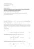
6 EURASIP Journal on Advances in Signal Processing 102 103 102 101 Polar RMSE (deg) Polar RMSE (deg) 101 100 100 10−1 10−1 10−2 10−2 10−3 10−3 −10 −10 0 10 20 30 40 0 10 20 30 40 SNR (dB) SNR (dB) 4λ 0.5λ 4λ 0.5λ 8λ 2λ 8λ 2λ (a) (b) Figure 2: Polarization state estimates RMSE of the proposed EVSA-PM against SNRs. (a) Source 1, (b) source 2. 102 102 101 101 DOA RMSE (deg) DOA RMSE (deg) 100 100 10−1 10−1 10−2 10−2 10−3 10−3 −10 0 10 20 30 40 −10 0 10 20 30 40 SNR (dB) SNR (dB) EVSA-PM (Δ = 4λ) EVSA-PM (Δ = 4λ) SUMWE SUMWE EVSA-PM (Δ = λ/ 2) CRB EVSA-PM (Δ = λ/ 2) CRB PSA-PM PSA-PM (a) (b) Figure 3: DOA estimate RMSEs of EVSA-PM, PSA-PM, and SUMWE against SNRs. (a) Source 1, (b) source 2. and the RMSE of kth source’s polarization state estimate is Figures 1 and 2 plot the RMSEs of the sources’ DOA and deﬁned as polarization estimates against signal-to-noise ratio (SNR) ⎧ levels using the EVSA-PM. The SNR is deﬁned as SNR = ⎛ ⎞ ⎪ 1⎨ 1 ⎝ E (1/K ) K=1 |sk |2 /σn , where σn is the noise power lever. Two 2 2 γe,k − γk ⎠ 2 RMSEk = ⎪ k 2 ⎩ E e=1 equal-power narrowband coherent signals impinge with parameters θ1 = 75◦ , ϕ1 = 35◦ , γ1 = 45◦ , η1 = −90◦ , θ2 = (27) ⎞⎫ 80◦ , ϕ2 = 30◦ , γ2 = 45◦ , and η2 = 90◦ , and the multipath ⎛ ⎪ ⎬ E coeﬃcient is set to β2 = exp( j ∗ 50◦ ). The uniform linear 1⎝ − ηk ⎠ , 2 + ηe,k ⎪ array consists of 12 six-component EmVSs. The intervector ⎭ E e=1 sensor spacing is set as Δ = Δ2 + Δ2 = 0.5λ, 2λ, 4λ, and x y 8λ, respectively. The snapshot number is 300. It is seen from where θe,k , ϕe,k , γe,k , and ηe,k symbolize the eth Monte that both DOA and polarization estimation errors decreases Carlo trial’s estimates for the kth source’s directions and polarization states and E is the total Monte Carlo trials. In as the SNR increases. Also, the increase of intervector the simulations, E = 500. sensor spacing, which results in the array aperture extension,
EURASIP Journal on Advances in Signal Processing 7 102 102 101 101 DOA RMSE (deg) DOA RMSE (deg) 100 100 10−1 10−1 10−2 10−2 101 102 103 101 102 103 Snapshot number Snapshot number EVSA-PM (Δ = 4λ) EVSA-PM (Δ = 4λ) SUMWE SUMWE EVSA-PM (Δ = λ/ 2) EVSA-PM (Δ = λ/ 2) CRB CRB PSA-PM PSA-PM (a) (b) Figure 4: DOA estimate RMSEs of EVSA-PM, PSA-PM and SUMWE against the number of snapshots. (a) Source 1, (b) source 2. 60 70 PSA-PM 60 EVSA-PM 50 50 40 40 30 30 20 20 10 10 0 0 65 66 67 68 69 70 71 72 73 74 75 65 66 67 68 69 70 71 72 73 74 75 Elevation angle Elevation angle (a) (b) 30 SUMWE 25 20 15 10 5 0 65 66 67 68 69 70 71 72 73 74 75 Elevation angle (c) Figure 5: The histogram of the estimated elevation using the three methods. (a) EVSA-PM; (b) PSA-PM; (c) SUMWE.
8 EURASIP Journal on Advances in Signal Processing contributes to the estimation accuracy enhancement. Since 120 the estimation of DOA and polarization is extracted from the EmVS steering vector, which contains no time-delay 100 phase factor, we can obtain more accurate but unambiguous Spatial spectrum (dB) 80 estimates of coherent source using an aperture extension array without a corresponding increase in hardware and 60 software costs [12]. 40 Figures 3 and 4 make the comparison between the proposed algorithm with PSA-PM and SUMWE under 20 diﬀerent SNRs and number of snapshots. The impinging 0 signal parameters are same as in Figures 1 and 2. We use 300 snapshots in Figure 3 and set SNR = 20 dB in Figure 4. −20 For the proposed algorithm, a uniform linear array with 8 dipole-triads, separated by Δ = λ/ 2 and 4λ is considered. −40 0 20 40 60 80 100 120 140 160 180 For the PSA-PM, we use an L-shape geometry, with 8 dipole- DOA (deg) triads uniformly placed along x-axis for estimating uk and 8 dipole-triads uniformly placed along y -axis for estimating PSA-FB-PM EVSA-PM PSA-PM SUMWE vk . For the SUMWE, we use an L-shape geometry, with 12 unpolarized scalar sensors uniformly placed along x- Figure 6: Spatial spectrum of EVSA-PM, PSA-PM, PSA-FB-PM, axis for estimating uk and 12 unpolarized scalar sensors and SUMWE for nine coherent sources. uniformly placed along y -axis for estimating vk . Hence, the hardware costs of the SUMWE and the presented algorithm are comparable. The intersensor displacement for the PSA- sensors [19] (i.e., N = 4, M = 20) for all the other PM and SUMWE is a half-wavelength, since these two three algorithms and estimate the sources’ direction by angle algorithms would suﬀer angle ambiguities when two sensors searching. The intervector sensor spacing of array is a half- are spaced over a half-wavelength. The curves in these two wavelength. Like [19], we assume zero elevation incident ﬁgures unanimously demonstrate that the proposed EVSA- angle (θk = 90◦ ) and randomly chosen polarizations for all PM with Δ = 4λ can oﬀer performance superior to those of sources, and set SNR = 15 dB. the PSA-PM and SUMWE. Nine equal power, coherent sources with the azimuth From the computational complexity analysis, the major incident angles 35◦ , 50◦ , 65◦ , 80◦ , 90◦ , 100◦ , 110◦ , 125◦ , computational costs involved in the three algorithms are the and 140◦ are considered, and the corresponding multipath calculation of the corresponding propagator and correlation coeﬃcients βk = exp( j ∗ 10◦ (k − 1)), k = 1, . . . , 9. This matrix, and the numbers of multiplications required by the ﬁgure shows that the proposed EVSA-PM and the SUMWE EVSA-PM, the PSA-PM, and SUMWE are in the order of successfully resolve the nine coherent signals, while the PSA- 2 O(3M1 KF + 18(M1 − 1)F ) ≈ 174F , O(2M1 KF + 6M1 F ) ≈ PM, and the PSA-FB-PM fail to do so. This is due to the 416F , and O(2M2 KF + 4(M2 − 1)F ) ≈ 92F , respectively, factor that the PSA-PM and the PSA-FB-PM, respectively, where M1 = 8, M2 = 12, and F denotes the number of only can resolve min(N , M − 1) = 4 and min(2N , M − 1) = 8 snapshots. Therefore, the proposed EVSA-PM also is more coherent sources at most, while the proposed EVSA-PM can computationally eﬃcient than the PSA-PM. resolve L − 2 coherent sources (L = M − K + 1), and the The proposed EVSA-PM can fully exploit polarization maximum number of coherent signals resolved using the diversity to resolve closely spaced sources with distinct SUMWE is equal to that using the EVSA-PM. polarizations. To verify this performance, we assume two incident coherent sources with parameters θ1 = 70◦ , θ2 = 70.5◦ , ϕ1 = 90◦ , ϕ2 = 90◦ , γ1 = 45◦ , γ2 = 45◦ , η1 = −90◦ , 5. Conclusions and η2 = 90◦ . Others simulation conditions are the same as This paper employs a linear electromagnetic vector-sensor that in Figure 4, except that the SNR is set at 35 dB. Figure 5 array to propose a novel pre-processing algorithm for shows the histogram of the estimated elevation using the decorrelating the coherent signals by electromagnetic vector- three methods based on 500 independent trials. From the sensor subarray averaging, and combine it with the propaga- ﬁgure, we can observe that the proposed EVSA-PM can tor method to estimate the DOA and polarization of coher- resolve the closely spaced sources. However, the other two ent sources without eigen-decomposition into signal/noise methods fail. subspaces. Compared with the existing estimate algorithms, Figure 6 plots the spatial spectrum to present comparison the proposed algorithm makes use of more available electro- of the maximum numbers of coherent signals, which can magnetic information, hence, has an improved estimation be, respectively, resolved by the proposed algorithm, the performance. It does not necessarily require the intervector SUMWE, the PSA-PM, and the PSA-FB-PM which combines sensor spacing of a half-wavelength, enable decorrelation of the PSA with the FB averaging technique [27]. We consider more coherent signals, and joint estimation of DOA and a uniform linear array comprised of 20 unpolarized scalar sensors for the SUMWE and 20 quadrature polarized vector polarization of coherent sources.
EURASIP Journal on Advances in Signal Processing 9 Appendix [9] C. Paulus and J. I. Mars, “Vector-sensor array processing for polarization parameters and DOA estimation,” EURASIP Journal on Advances in Signal Processing, vol. 2010, Article ID From (12), we can obtain 850265, 3 pages, 2010. def [R1 , . . . , R6 ] = AFG, (A.1) [10] Y. Xu, Z. Liu, K. T. Wong, and J. Cao, “Virtual-manifold ambi- guity in HOS-based direction-ﬁnding with electromagnetic def where F = diag (rs1 β1 , . . . , rs1 βK1 , rsK1 +1 qM (θK1 +1 , ϕK1 +1 ), . . . , vector-sensors,” IEEE Transactions on Aerospace and Electronic rsK qM (θK , ϕK )) Systems, vol. 44, no. 4, pp. 1291–1308, 2008. ⎡ ⎤ [11] K. T. Wong and M. D. Zoltowski, “Closed-form direction ρM,1 hT ρM,2 hT ρM,6 hT ... 1 1 1 ﬁnding and polarization estimation with arbitrarily spaced ⎢ ⎥ ⎢ ⎥ electromagnetic vector-sensors at unknown locations,” IEEE ⎢ ⎥ . . . .. . . . ⎢ ⎥ . . . . ⎢ ⎥ Transactions on Antennas and Propagation, vol. 48, no. 5, ⎢ ⎥ ⎢ ρ hT ρM,6 hT 1 ⎥ pp. 671–681, 2000. ρM,2 hT 1 def ⎢ ⎥ ... M,1 K1 K K ⎢ ⎥ [12] M. D. Zoltowski and K. T. Wong, “ESPRIT-based 2-D direc- G=⎢ ⎥ ⎢c1,K1 +1 hT +1 c2,K1 +1 hT +1 c6,K1 +1 hK1 +1 ⎥, T tion ﬁnding with a sparse uniform array of electromagnetic ... ⎢ ⎥ K1 K1 ⎢ ⎥ vector sensors,” IEEE Transactions on Signal Processing, vol. 48, ⎢ ⎥ . . . .. ⎢ ⎥ . . . no. 8, pp. 2195–2204, 2000. . ⎢ ⎥ . . . ⎣ ⎦ [13] K. T. Wong, “Blind beamforming geolocation for wideband- c1,K hT c2,K hT c6,K hT ... FFHs with unknown hop-sequences,” IEEE Transactions on K K K Aerospace and Electronic Systems, vol. 37, no. 1, pp. 65–76, def T hk = q1 θk , ϕk , . . . , qK θk , ϕk 2001. . [14] H. Jiacai, S. Yaowu, and T. Jianwu, “Joint estimation of DOA, (A.2) frequency, and polarization based on cumulants and UCA,” The matrix A is of full column rank due to the distinct Journal of Systems Engineering and Electronics, vol. 18, no. 4, pp. 704–709, 2007. polarizations (although there are two sources from the same [15] K. C. Ho, K. C. Tan, and A. Nehorai, “Estimating direc- direction). The diagonal matrix F has full rank. If the two tions of arrival of completely and incompletely polarized sources have the same incident directions but with the signals with electromagnetic vector sensors,” IEEE Transac- distinct polarizations, and are uncorrelated with each other tions on Signal Processing, vol. 47, no. 10, pp. 2845–2852, (i.e., the two sources are not all included in the set consisting 1999. of the ﬁrst K1 coherent sources), the K ×6K matrix G is of full [16] K. T. Wong and M. D. Zoltowski, “Uni-vector-sensor ESPRIT row rank. Therefore, in this scenario, the matrix [R1 , . . . , R6 ] for multisource azimuth, elevation, and polarization estima- is of rank K . Similarly, the matrix [R1 , . . . , R6 ] also is of rank tion,” IEEE Transactions on Antennas and Propagation, vol. 45, K . Thus, the matrix R deﬁned in (11) still has full rank. no. 10, pp. 1467–1474, 1997. [17] K. T. Wong and M. D. Zoltowski, “Self-initiating MUSIC- References based direction ﬁnding and polarization estimation in spatio- polarizational beamspace,” IEEE Transactions on Antennas and [1] A. Nehorai and E. Paldi, “Vector-sensor array processing for Propagation, vol. 48, no. 8, pp. 1235–1245, 2000. electromagnetic source localization,” IEEE Transactions on [18] M. D. Zoltowski and K. T. Wong, “Closed-form eigenstruc- Signal Processing, vol. 42, no. 2, pp. 376–398, 1994. ture-based direction ﬁnding using arbitrary but identical [2] J. Li, “Direction and polarization estimation using arrays with subarrays on a sparse uniform Cartesian array grid,” IEEE small loops and short dipoles,” IEEE Transactions on Antennas Transactions on Signal Processing, vol. 48, no. 8, pp. 2205–2210, and Propagation, vol. 41, no. 3, pp. 379–386, 1993. 2000. [3] K. T. Wong, “Direction ﬁnding/polarization estimation— [19] D. Rahamim, J. Tabrikian, and R. Shavit, “Source localization dipole and/or loop triad(s),” IEEE Transactions on Aerospace using vector sensor array in a multipath environment,” IEEE and Electronic Systems, vol. 37, no. 2, pp. 679–684, 2001. Transactions on Signal Processing, vol. 52, no. 11, pp. 3096– [4] B. Hochwald and A. Nehorai, “Polarimetric modeling and 3103, 2004. parameter estimation with applications to remote sensing,” [20] Y. Wu, H. C. So, C. Hou, and J. Li, “Passive localization of IEEE Transactions on Signal Processing, vol. 43, no. 8, pp. 1923– near-ﬁeld sources with a polarization sensitive array,” IEEE 1935, 1995. Transactions on Antennas and Propagation, vol. 55, no. 8, [5] X. Gong, Z. Liu, Y. Xu, and M. Ishtiaq Ahmad, “Direction- pp. 2402–2408, 2007. of-arrival estimation via twofold mode-projection,” Signal [21] M. Kanda and D. A. Hill, “A three-loop method for deter- Processing, vol. 89, no. 5, pp. 831–842, 2009. mining the radiation characteristics of an electrically small [6] J. Tabrikian, R. Shavit, and D. Rahamim, “An eﬃcient vector source,” IEEE Transactions on Electromagnetic Compatibility, sensor conﬁguration for source localization,” IEEE Signal vol. 34, no. 1, pp. 1–3, 1992. Processing Letters, vol. 11, no. 8, pp. 690–693, 2004. [22] R. O. Schmidt, “Multiple emitter location and signal param- [7] S. Miron, N. Le Bihan, and J. I. Mars, “Quaternion-MUSIC for eter estimation,” IEEE Transactions on Antennas and Propaga- vector-sensor array processing,” IEEE Transactions on Signal tion, vol. 34, no. 3, pp. 276–280, 1986. Processing, vol. 54, no. 4, pp. 1218–1229, 2006. [8] C. C. Ko, J. Zhang, and A. Nehorai, “Separation and tracking [23] R. Roy and T. Kailath, “ESPRIT—estimation of signal parame- of multiple broadband sources with one electromagnetic ters via rotational invariance techniques,” IEEE Transactions on Acoustics, Speech, and Signal Processing, vol. 37, no. 7, pp. 984– vector sensor,” IEEE Transactions on Aerospace and Electronic 995, 1989. Systems, vol. 38, no. 3, pp. 1109–1116, 2002.
10 EURASIP Journal on Advances in Signal Processing [24] N. Tayem and H. M. Kwon, “L-shape 2-dimensional arrival angle estimation with propagator method,” IEEE Transactions on Antennas and Propagation, vol. 53, no. 5, pp. 1622–1630, 2005. [25] C. Gu, J. He, X. Zhu, and Z. Liu, “Eﬃcient 2D DOA estimation of coherent signals in spatially correlated noise using electro- magnetic vector sensors,” Multidimensional Systems and Signal Processing, vol. 21, no. 3, pp. 239–254, 2010. [26] J. Xin and A. Sano, “Computationally eﬃcient subspace- based method for direction-of-arrival estimation without eigendecomposition,” IEEE Transactions on Signal Processing, vol. 52, no. 4, pp. 876–893, 2004. [27] S. U. Pillai and B. H. Kwon, “Forward/backward spatial smoothing techniques for coherent signal identiﬁcation,” IEEE Transactions on Acoustics, Speech, and Signal Processing, vol. 37, no. 1, pp. 8–15, 1989.