Báo cáo hóa học: "Research Article Epileptic Seizure Prediction by a System of Particle Filter Associated with a Neural Network"

Chia sẻ: Linh Ha | Ngày: | Loại File: PDF | Số trang:10

Thêm vào BST

Báo xấu

74
lượt xem 4
download

Download Vui lòng tải xuống để xem tài liệu đầy đủ

Tuyển tập báo cáo các nghiên cứu khoa học quốc tế ngành hóa học dành cho các bạn yêu hóa học tham khảo đề tài: Research Article Epileptic Seizure Prediction by a System of Particle Filter Associated with a Neural Network

Chủ đề:

Bình luận(0) Đăng nhập để gửi bình luận!

Lưu

Nội dung Text: Báo cáo hóa học: "Research Article Epileptic Seizure Prediction by a System of Particle Filter Associated with a Neural Network"

Hindawi Publishing Corporation EURASIP Journal on Advances in Signal Processing Volume 2009, Article ID 638534, 10 pages doi:10.1155/2009/638534 Research Article Epileptic Seizure Prediction by a System of Particle Filter Associated with a Neural Network Derong Liu,1 Zhongyu Pang,2 and Zhuo Wang2 1 The Key Laboratory of Complex Systems and Intelligence Science, Institute of Automation, Chinese Academy of Sciences, Beijing 100190, China 2 Department of Electrical and Computer Engineering, University of Illinois at Chicago, Chicago, IL 60607-7053, USA Correspondence should be addressed to Derong Liu, derong.liu@ia.ac.cn Received 3 December 2008; Revised 5 March 2009; Accepted 28 April 2009 Recommended by Jose Principe None of the current epileptic seizure prediction methods can widely be accepted, due to their poor consistency in performance. In this work, we have developed a novel approach to analyze intracranial EEG data. The energy of the frequency band of 4–12 Hz is obtained by wavelet transform. A dynamic model is introduced to describe the process and a hidden variable is included. The hidden variable can be considered as indicator of seizure activities. The method of particle ﬁlter associated with a neural network is used to calculate the hidden variable. Six patients’ intracranial EEG data are used to test our algorithm including 39 hours of ictal EEG with 22 seizures and 70 hours of normal EEG recordings. The minimum least square error algorithm is applied to determine optimal parameters in the model adaptively. The results show that our algorithm can successfully predict 15 out of 16 seizures and the average prediction time is 38.5 minutes before seizure onset. The sensitivity is about 93.75% and the speciﬁcity (false prediction rate) is approximately 0.09 FP/h. A random predictor is used to calculate the sensitivity under signiﬁcance level of 5%. Compared to the random predictor, our method achieved much better performance. Copyright © 2009 Derong Liu et al. This is an open access article distributed under the Creative Commons Attribution License, which permits unrestricted use, distribution, and reproduction in any medium, provided the original work is properly cited. 1. Introduction epilepsy will continue to experience seizures even with the best available treatment [1]. Epilepsy is a brain disorder in which neurons in the brain EEG can be used to record brain waves detected by produce abnormal signals. One explanation for epilepsy is electrodes placed on the scalp or on the brain surface. that neuronal activity of human brain has two patterns. One This is the most common diagnostic test for epilepsy and is the normal pattern which corresponds to normal activities can detect abnormalities in the brain’s electrical activity. while the other is abnormal pattern in which epilepsy is Some nonlinear measurement methods such as dimensions, Lyapunov exponents, and entropies were shown to oﬀer new included. Neuronal activity of epilepsy can cause various abnormal situations such as strange sensations, emotions information about complex brain dynamics and further to and behavior and loss of consciousness. Possible reasons predict seizure onset. causing epilepsy are not unique. Seizure and epilepsy are not Iasemidis et al. [2, 3] were pioneers in making use completely equivalent. That is, a person having a seizure does of nonlinear dynamics to analyze clinical epilepsy. Their not necessarily mean that he/she has epilepsy. According to method was based on the assumption that there was a the medical deﬁnition of epilepsy, the condition is that a transition from normal brain activity to a seizure occurrence. person with epilepsy should have two or more seizures in a Thus, state changes could indicate seizure occurrence. In time period. 2003 [1], they showed that it was possible to predict Based on information from the National Institutes of seizures minutes or even hours in advance by using the Health, about 1 in 100, or more than 2 million people in spatiotemporal evolution of shortterm largest Lyapunov the United States, has experienced an unprovoked seizure exponent on multiple regions of the cerebral cortex, since or been diagnosed with epilepsy. About 20% of people with seizure could be characterized by similarity of chaotical
2 EURASIP Journal on Advances in Signal Processing degree of their dynamical states. Later on, an adaptive seizure predictor generates alarms following a Poisson process in prediction algorithm was developed to analyze continuous time without using any information from the EEG [10]. EEG recordings with temporal lobe epilepsy for the purpose The sensitivity from the random predictor can be obtained. of prediction when only the occurrence of the ﬁrst seizure is Comparing the two, our prediction results are superior to known [4]. those from the random predictor. There are many researchers who are working in this This paper is organized as follows. In Section 2, we ﬁeld and many publications have appeared. Ebersole [5] introduce particle ﬁlters and neural networks. In Section 3, summarized some seizure prediction methods from the First our method is presented including the dynamic model International Collaborative Workshop on Seizure Prediction and the way for solving the hidden variable. In Section 4, (2005). He believed that no seizure forewarning has been experimental data is given. In Section 5, data processing realized into the clinic. Hassanpour et al. [6] estimated and simulation results are described. Finally, in Section 6, the distribution function of singular vectors based on the discussion and conclusions are addressed. time frequency distribution of an EEG epoch to detect the patterns embedded in the signal. Then they trained a 2. Particle Filters neural network and further discriminate between seizure and nonseizure patterns. Mormann et al. [7] summarized some Although particle ﬁlters, namely, sequential Monte Carlo prediction methods and pointed out some of their pitfalls. methods, were introduced much earlier, it became attractive They also summarized the current state of this research ﬁeld and was further developed in the 1990s since comput- and possible future development. In order to improve the ers can provide more powerful ability of computation. performance of an algorithm, a better understanding of the These methods have been very popular over the past inter-ictal period is necessary and all of its confounding few years in statistics and related ﬁelds since it can be variables should inﬂuence the characterizing measures used used to simulate nonlinear non-Gaussian distributions, and in the algorithms. They mentioned that a further promising they are improved greatly in the implementation [12–17]. approach would be to model EEG signals to gain insight into Particle ﬁlters can approximate a sequence of probability the dynamical processes involved in seizure generation [8], distributions of interest using a set of random samples [9]. For purpose of comparison, Schelter et al. [10] estimated called particles. These particles are propagated over time the performance of a seizure prediction method based following the corresponding distributions by sampling and on a quantity indicating phase synchronization compared resampling mechanisms. At any time, as the number of with a Poisson process. Using invasive EEG data of four particles increases, particles should asymptotically converge representative patients suﬀering from epilepsy, they claimed toward the sequence of theoretical probability distribution. that two of them have good performance while the other In reality, computation time is a very important factor to two do not. Therefore, further research in this ﬁeld is still consider so the number of particles cannot go too big. necessary. Thus eﬀective sampling algorithms are key steps to capture In this work, we use a nonlinear method diﬀerent a certain probability distribution by a limited number of from existing ones to predict seizures. We believe that EEG particles. measurements of seizures from epileptic patients can be The basis of a particle ﬁlter is a sequential importance described as a stochastic process and has a certain probability sampling/resampling algorithm [18]. Most sequential Monte distribution. Suﬀczynski et al. [8] investigated the dynamical Carlo methods developed over the last decade are based on transitions between normal and paroxysmal state of epilepsy. this algorithm. This technique is capable of implementing a A Poisson process or a random walk process can be used recursive Bayesian ﬁlter by Monte Carlo simulations. The key to simulate the transition between the two states. We found idea is to use a sample of random particles to approximate a that the characteristic variables from epileptic EEG data can posterior probability distribution. The sequential sampling be used to represent the procedure of seizure occurrence. is very important in realizing this algorithm. Assume an We develop a dynamic model where a hidden variable arbitrary distribution p(x). Samples are supposed to be is involved. Features of the hidden variable can become drawn from p(x), but in many practical cases, p(x) is not an indicator of seizure occurrence. The hidden variable is a standard probability distribution,for example, Gaussian considered to have the property of second order Markov distribution, and, therefore, it is diﬃcult to draw samples chain. The method of particle ﬁlter associated with a neural from p(x). Based on the Bayesian importance sampling network is used to estimate the hidden variable. Features of scheme [19], a sample xi , i = 1, . . . , N , can be drawn from the hidden variable can be extracted and seizure onset can another probability distribution q(x) called the importance be detected in advance based on these features. As pointed function, which is easy to sample. Thus these particles out by Litt et al. [11], during the transition from normal can approximate the distribution q(x). In order to use brain activities to a seizure, some regions of the brain have these particles to represent the desired distribution p(x), a similar activities. This similarity makes it possible for some weighted approximation to the density p(x) is given by characteristics detectable during the preseizure period. Based on a probability distribution, the sensitivity can be reached by a random predictor. It is meaningful only when a N i=1 w δ x − x i i predictor has higher sensitivity than the random predictor. p (x ) = , (1) N i i=1 w We set signiﬁcance level as 5%. Assume that the random
EURASIP Journal on Advances in Signal Processing 3 particles. In (7), the term p(αn | α1:n−1 ) is omitted since it is where a value by calculation. Doucet [21] showed that the eﬀect of xi p omission is compensated by normalizing the weights using wi = , (2) q(xi ) i wn i wn = . (9) and δ (·) is a Dirac delta function deﬁned as N i i=1 wn ⎧ The sequential importance sampling algorithm has been ⎨1, if x = xi i δ x−x = developed, but two problems exist in practice. One is the (3) ⎩ 0, otherwise. phenomenon of degeneracy and the other is the choice of importance function q(x). In general, all but a few particles If the samples are drawn from an importance function will have negligible weights after several iterations and a q(x1:n | α1:n ), then the weights in (2) are determined as large computational eﬀort is devoted to updating trajectories whose contribution to the ﬁnal estimation is almost zero i p x1:n | α1:n [18]. Liu and Chen [16] introduced a method to measure wi = . (4) particle degeneracy. The eﬀective sample size Neﬀ is deﬁned q(x1:n | α1:n ) as: Now we can proceed to obtain a recursive updating Ns Neﬀ = , (10) equation which can keep the previous trajectories of particles ∗ 1 + Var wn i when a set of new data is available. At each iteration, ∗ where wn i denotes the true weight by calculation directly. It samples can approximate the corresponding distribution,for example, p(x1:n−1 | α1:n−1 ), and then approximate p(x1:n | is not easy to calculate Neﬀ from the above equation, so an approximation of Neﬀ can be used as α1:n ) with a new set of samples. From the Bayesian theory, we can easily obtain 1 Neﬀ = 2, (11) Ns i wn q(x1:n | α1:n ) = q(xn | x1:n−1 , α1:n )q(x1:n−1 | α1:n−1 ). i=1 (5) i where wn is the normalized weight obtained from (8). i From (5), we already have samples x1:n−1 ∼ q(x1:n−1 | The smaller the Neﬀ , the worse the degeneracy. Generally α1:n−1 ), and can draw a particle from xn ∼ q(xn | i speaking, increasing the number of particles can reduce i x1:n−1 , α1:n ) to augment samples to become x1:n . The aim is degeneracy, but it is impractical. When Neﬀ ≤ Nthreshold , to approximate density function p(·), and p(x1:n | α1:n ) is where Nthreshold is usually taken as one third of the particle number, resampling is necessary. Resampling procedures expressed as follows, based on the Bayesian theory and the can decrease the degeneracy phenomenon but it introduces Markov properties [20], practical, and theoretical problems [18]. From a theoretical p(αn | xn ) p(xn | xn−1 ) point of view, the simulated trajectories are no longer p(x1:n | α1:n ) = p(x1:n−1 | α1:n−1 ). p(αn | α1:n−1 ) statistically independent after resampling so the previous (6) convergence result will be lost. From a practical point of view, it limits the opportunity to parallel computation since When particle weights are considered, the updating all the particles must be combined, although the importance equation is given by sampling steps can still be realized in parallel. i i p αn | xn p xn | xn−1 p x1:n−1 | α1:n−1 i i 3. Methods i wn = i i q xn | x1:n−1 , α1:n q x1:n−1 | α1:n−1 p(αn | α1:n−1 ) i This section includes three parts. The ﬁrst part describes our dynamic model. The second one introduces the solution for i i p αn | xn p xn | xn−1 p x1:n−1 | α1:n−1 i i ∝ hidden variable in our model. The last one addresses seizure i i q xn | x1:n−1 , α1:n x1:n−1 | α1:n−1 i feature selection and determination. i p αn | xn p xn | xn−1 i i 3.1. Dynamic Model. Energy can be used to represent i = wn−1 . features of a signal. For epileptic seizures, we ﬁnd that energy i | i q xn x1:n−1 , α1:n for some speciﬁc frequency band (4–12 Hz), which includes (7) theta (4–8Hz) and alpha (8–12 Hz) waves, can be modeled by a similar Poisson process. Other combinations based on Based on the prior distribution, the initial step of the delta (0–4 Hz), theta, alpha, and beta (12–30 Hz) waves are above recursion can be deﬁned for n = 1 as also calculated but their characteristics are not as obvious. p(x1 | α1 ) Our dynamic state model is given by i w1 = . (8) q(x1 | α1 ) xk = αxk−1 + βxk−2 + vk (12) Thus, particle weights for n = 1, 2, . . ., can recursively Ek = Axk e−xk /B + wk , k = 1, 2, . . . , be obtained. We can extend the same procedure to all the
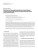
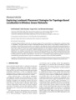
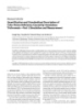
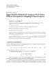
4 EURASIP Journal on Advances in Signal Processing where xk is a random variable and has a normal dis- seizure. A and B can be obtained by minimizing error wk . tribution initially. vk , wk are white noise with Gaussian One further step is to do regression analysis. distribution and they are independent. α, β are parameters The regression analysis is based on the method of to be determined. Ek is the energy from speciﬁc frequency Chatterjee and Hadi [24], expressed by band. A and B are unknown constants. The process for xk ∼ N 0, σ 2 I , Y = Xξ + , (14) is actually assumed to be a second-order Markov chain. The where Y is a dependent variable (output), X is an inde- hidden variable xk can represent transition changes and has pendent variable (input or data), and is the error. The the ability to indicate seizure occurrence in advance. The parameter ξ can be determined using the least square error process chosen in (12) is based on our study and on the method and the predicted data can then be obtained from work in [8]. Also, the energy in a frequency band changes continuously and its value is aﬀected by the most recent past (14). Normally there is a peak at some time instants before values. To the best of our knowledge, no other researchers seizure occurrence and x value will be between 270 and have developed a model which is used to simulate seizure 360 during the ictal period. The feature of a “peak” can process behaviors and further to predict their occurrence. be described by the mean value (with threshold of ±10% of the previous mean value), the variance before it (with 3.2. Solution of the Dynamic Model. We already introduced threshold of ±5% of the mean of previous variance), the peak particle ﬁlters in Section 2. In order to improve its perfor- amplitude (at least 10 more than the previous mean value), mance under small number of particles, we develop a novel and the width of peak (from 1 minute to 6 minutes). The algorithm to combine particle ﬁlters with neural networks. mean value and variance can be calculated for 15–30 minutes The strategy of backpropagation neural networks can be used before the peak; peak amplitude can be detected by the real to adjust particles in tail area with low weights in a particle peak value, and the width of peak can also be obtained at ﬁlter. the same time. We assume that these features will be kept the The basic idea of backpropagation neural networks is to same at the next seizure onset. All the features can be updated use the steepest descent (gradient) procedure to minimize as long as the information of a new seizure is available. the error energy at the output layer. The error energy can be Thus the system can adaptively update all related parameters denoted as follows: automatically based on available seizure information. From Figure 1, the hidden variable’s value at certain time 1 1 Δ 2 ek 2 , E= dk − yk = (13) before seizure occurrence reaches a peak. Before that peak, 2 2 k k the variance is small, which means that the curve before the peak is smooth. Figure 1 shows this characteristic. The where k = 1, . . . , N ; N is the number of neurons in the output diﬀerence between the time at which seizure is alerted to layer. dk is the target value and yk is the output of neural happen, and seizure actual occurrence is the prediction time. network. By using gradient procedure and updating weights Based on this type of signature, a certain time point before of all neurons to train a neural network, proper weights can seizure occurrence can be recognized and a seizure alert is be found so that the output of the network is close to the provided at that point. For Figure 1, the prediction time is 14 desired objective within an assigned error. The activation minutes. The minimum intervention time is set to 2 hours function in neural networks can be chosen according to in our study. If a seizure appears from 3 to 120 minutes actual problems [22]. after a seizure is alerted, this prediction is considered to be There are one input, one hidden, and one output layer successful. Otherwise, a false prediction is counted. built in our algorithm. The dimension of input layer is determined adaptively by particle samples in the particle 4. Experimental Data ﬁlter. Particles with smaller weights are considered as the input data of a neural network. Their corresponding weights The EEG data that we use are invasive EEG recordings of 6 are set as inputs of the neural network, and their particle patients with medically intractable temporal lobe epilepsy. values as initial weights of the neural network. The weights The data were recorded during an invasive presurgical of the remaining particles are set as biases of corresponding epilepsy monitoring at the Epilepsy Center of the University neurons. The neural networks can improve the performance Hospital of Freiburg, Germany. In order to obtain a high of particle ﬁlters,for example, the number of simulation is signal-to-noise ratio, fewer artifacts, and to record directly reduced signiﬁcantly. The noise wk in (12) is small since from temporal areas, intracranial grid-, strip-, and depth- measurements are intracranial EEG data. In general, the electrodes were utilized. The EEG data were acquired computational complexity is O(N ), where N is the number using a Neuroﬁle NT digital video EEG system with 128 of particles. Our algorithm is displayed in Algorithm 1 [23]. channels, 256 Hz sampling rate, and a 16 bit analog-to-digital converter. For each patient, we were given 4–6 channels of 3.3. Feature Determination. Based on Algorithm 1, the hid- data recorded from temporal areas. The amplitude of data den variable in the dynamic model can be obtained. For a is relative to the real one after sampling them, but all the given patient, suppose that the ﬁrst seizure is known. All features will be kept the same. the parameters in (12) can be obtained. Parameters α and β For each patient, there are datasets called “ictal,” and can be determined by minimizing errors, based on a known “interictal,” with the former containing EEG-recordings with
EURASIP Journal on Advances in Signal Processing 5 1. Importance sampling Δ i i -For i = 1, . . . , N , sample xn ∼ q(xn | x1:n−1 , α1:n ), and set x1:n = (x1:n−1 , xn ), i i i where q(xn | x1:n−1 , α1:n ) is a chosen probability density function. N is the number of particles and n is the current time. -For i = 1, . . . , N , evaluate the importance weights up to a normalizing constant: i ii i i wn = wn−1 ( p(αn xn ) p(xn xn−1 ))/q(xn | x1:n−1 , α1:n ), where p(αn | xn ), and p(xn | xn−1 ) i i i i i i are conditional probability density functions for αn , and xn , respectively. -For i = 1, . . . , N , normalize the importance weights: j wn = wn / N=1 wn ,where wn is the normalized weight. i i i j -At time n, identify particles with high weights, and low weights. Replace some low weight particles with high ones if needed. -At time n, adjust particles with low weights by neural networks. Assign and normalize weights by the aforementioned procedure i2 -Evaluate Neﬀ using Neﬀ = 1/ Ns1 (wn ) , where Neﬀ is the threshold parameter. i= 2. Resampling if necessary i i -If Neﬀ ≥ Nthreshold , where Nthreshold is a preset threshold, x1:n = x1:n for i = 1, . . . , N ; -Otherwise, for i = 1, . . . , N , sample an index j (i) distributed according to the discrete distribution with N elements satisfying Pr { j (i) = l} = wn for l = 1, . . . , N ; l j (i) ∗i ∗ i for i = 1, . . . , N , x1:n = x1:n , and wn = 1/N , where wn i is an updated weight. Algorithm 1: Importance sampling/resampling particle ﬁlter with a neural network. epileptic seizures, and the latter EEG-recordings without One seizure with predition time 380 seizure activity. We use all ictal EEG data, and at least 10 hours interictal data for each subject. 360 For a particle ﬁlter, the optimal strategy is to choose i i q(xn | xn−1 , αn ) = p(xn | xn−1 ). Therefore, we use 340 linearization technique to linearize the model (12). It now becomes x variable 320 xk = αxk−1 + βxk−2 + vk = f (xk−1 , xk−2 ) + vk , (15) 300 Ek = A f (xk−1 , xk−2 )e− f (xk−1 ,xk−2 )/B Prediction time 280 + Axk e−xk /B − Axk e−xk /B /B |xk = f (xk−1 ,xk−2 ) (16) 260 Seizure onset × xk − f (xk−1 , xk−2 ) + wk , k = 1, 2, . . . . 240 0 5 10 15 20 25 30 35 40 45 50 Time (minutes) 5. Results Figure 1: One typical ﬁgure with prediction time and seizure. The vertical solid line marks prediction time point and the vertical 5.1. Data Preprocessing. Intracranial EEG data are unpro- dashed line indicates seizure occurrence. cessed directly from patients. Although they were obtained from intracranial electrode contacts on brain directly, there still exist some unusual values in the recording,for exam- ple, very big diﬀerence between two close points in the 5.2. Preprocessing. Based on the dynamic model (12), Ek is obtained from the above steps and the hidden variable xk can measurement. These points can be replaced with normal ones by interpolation, since there are few of this type of be found by particle ﬁlter associated with a neural network points in our data. Then roll-over windowing technique is realized by Algorithm 1. We assume that the initial condition of xk for the model is a normal distribution N (300, 5). The applied to them. We choose nonoverlap 5-second window to divide EEG data of a single channel. Wavelet transform mean value that we choose is based on initial energy that we “DB4” is used to get the energy of speciﬁc band since calculate. Normally its value is about 300. Thus, less time is it can give good performance and it is widely used to needed to run Algorithm 1 at the initial points. Actually this analyze EEG data. Compared with energy of diﬀerent value cannot have any eﬀect on the ﬁnal result except the running time. vk , wk are white noise, and we assume vk ∼ frequency bands, the frequency band of 4–12 Hz shows N (0, 0.6) and wk ∼ N (0, 0.1). In the dynamic model (12), much better performance and is chosen for use in our A, B are unknown parameters. The number of particles that model.
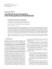
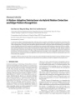
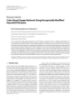
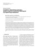
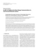
6 EURASIP Journal on Advances in Signal Processing Table 1: The optimal parameters α and β for six patients One seizure with prediction time 380 Patient No. No. 1 No. 2 No. 3 No. 4 No. 5 No. 6 α 0.7972 0.9001 0.8164 0.8775 0.9155 0.8599 360 β 0.2028 0.0999 0.1846 0.1225 0.0845 0.1401 340 x value we use is 200. For each patient, the ﬁrst seizure is supposed 320 to be known and is used to determine the parameters. The 300 algorithm of minimum least squares error is used to ﬁnd the optimal parameters under the assumption that the process is 280 steady before the next seizure occurrence. We follow the same procedure when dealing with all seizures of each patient. 260 According to the energy values calculated and parameter optimization, A = 2800 and B = 40 can be obtained. Table 1 240 0 5 10 15 20 25 30 35 40 45 50 55 60 shows the optimal parameters α and β for six patients based Time (minutes) on the ﬁrst seizure occurrence. Model (12) is a nonlinear model with Gaussian state (a) space. A local linearization technique is applied to nonlinear Interictal EEG without seizure equations and an approximate linear equation is obtained in 380 (16). A series of values of hidden variable x can be obtained based on Algorithm 1. 360 5.3. Experimental Results. Intracranial EEG data from six 340 patients are tested using our algorithm. It includes a total x value 320 of 22 epileptic seizures, and 110 hours of data. Six of them are taken out to determine all the related parameters in 300 model (12) for the subsequent seizures of each patient. After the preprocessing described above, Algorithm 1, namely, the 280 particle ﬁlter associated with a neural network, is used to identify the hidden variable x. In order to recognize 260 the general characteristics before seizure onset, the method 240 of linear regression is applied to calculated values of x. 0 5 10 15 20 25 30 35 40 45 50 55 60 This regression process can make clear the tendency of Time (minutes) change for the hidden variable x and provide some obvious (b) characteristics which are used to identify seizure occurrence in advance. Figure 2: Ictal and interictal hidden variable x from one patient Figures 2–7 show the hidden variable x from six patients with epilepsy. The vertical solid line marks prediction time point computed by our algorithm. Each of them includes two and the vertical dashed line indicates seizure occurrence. ﬁgures, one from ictal EEG with one seizure, and the other from interictal EEG without seizure. It is seen for all the ictal EEG that the characteristics occurring some time instants before the seizure can be recognized and used for predicting seizure onset. All patients here have temporal lobe epilepsy. prediction times are 39 and 38.5 minutes, respectively. Figure Figure 2 shows an epileptic seizure from a male patient. The 7 comes from a young male patient. Both ictal and interictal values x are relatively low compared to other patients, but prediction time is 42 minutes. After seizure happens, the variable x is on a little high level compared to that before its characteristics before the seizure are obvious. This seizure seizure. For the interictal period, the value x is higher than can be known 6.25 minutes in advance. that during ictal period. Figure 3 shows an epileptic seizure Totally we tested 16 seizures from these 6 patients. from a female patient. Its characteristics are the same as The average prediction time is 38.5 minutes. The longest Figure 2 including ictal and interictal transition data. The prediction time is 83.7 minutes and the shortest one is prediction time is about 11.5 minutes. Data in Figure 4 are 6.25 minutes. 15 seizures can be predicted successfully. The sensitivity is 93.75%.101 hours intracranial EEG testing data from a female patient too. The prediction time is about 30 minutes. The interictal characteristics, which oscillate on the are analyzed by our algorithm and speciﬁcity (false-positive low values, are diﬀerent from others. Figures 5 and 6 have rate) is about 0.09 FP/hour. very similar characteristics: ﬁgures for interictal EEG data In order to determine the performance of our method, are on the relative low values smoothly; ﬁgures for ictal EEG a random predictor is used to calculate the sensitivity. We data are on similar values. Figure 5 is from a young male assume that the random predictor generates alarms following patient and Figure 6 is from an old female patient. Their a Poisson process in time without using any information
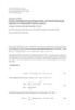
EURASIP Journal on Advances in Signal Processing 7 One seizure with prediction time One seizure with prediction time 420 370 360 400 350 380 340 330 360 x value x value 320 340 310 320 300 290 300 280 280 270 260 260 0 5 15 20 25 30 35 40 45 50 0 5 10 15 20 25 30 35 40 45 50 Time (minutes) Time (minutes) (a) (a) Interictal EEG without seizure Interictal EEG without seizure 420 360 400 340 380 320 360 300 x value x value 340 280 320 260 300 240 280 220 200 260 0 5 10 15 20 25 30 35 40 45 50 55 60 0 5 10 15 20 25 30 35 40 45 50 55 60 Time (minutes) Time (minutes) (b) (b) Figure 4: Ictal and interictal hidden variable x from one patient Figure 3: Ictal and interictal hidden variable x from one patient with epilepsy. The vertical solid line marks prediction time point with epilepsy. The vertical solid line marks prediction time point and the vertical dashed line indicates seizure occurrence. and the vertical dashed line indicates seizure occurrence. from the EEG. The probability to raise an alarm in a period This is the probability of predicting at least k out of K of duration can be calculated as [10] seizures by means of at least one of d independent features correctly. For our case, d is one. The signiﬁcance level is P ≈ RFP × PSO , (17) set at 5%. For 2 seizures, the sensitivity is 100% to meet the signiﬁcance level. The sensitivity is 67% for 3 seizures when RFP × PSO is smaller than one, where RFP is the and it is 50% for 4 seizures. Our method can detect 15 out maximum false prediction rate, which is set as 2 seizures each of 16 seizures, and the only one missed is from a patient day, and PSO is seizure occurrence period. In our case, PSO having 4 seizures. For 5 out of the 6 patients, our method is 2 hours. To decide the statistical signiﬁcance of sensitivity has sensitivity of 100%. The sensitivity for the other patient values, we follow Schelter’s method [10] to calculate the with a missed detection is 75% which is much better than probability as the random predictor (which is only 50%). Therefore, our ⎛ ⎛⎞ ⎞d method has superior performance to the random predictor. K =1−⎝ ⎝ ⎠P j P K − j ⎠ , (18) P{k;K ;P} j 6. Discussions and Conclusions j
8 EURASIP Journal on Advances in Signal Processing One seizure with prediction time One seizure with prediction time 400 400 380 380 360 360 x value x value 340 340 320 320 300 300 280 280 0 5 10 15 20 25 30 35 40 45 50 55 60 0 5 10 15 20 25 30 35 40 45 50 55 60 Time (minutes) Time (minutes) (a) (a) Interictal EEG without seizure Interictal EEG without seizure 400 400 380 380 360 360 x value x value 340 340 320 320 300 300 280 280 0 5 10 15 20 25 30 35 40 45 50 55 60 0 5 10 15 20 25 30 35 40 45 50 55 60 Time (minutes) Time (minutes) (b) (b) Figure 5: Ictal and interictal hidden variable x from one patient Figure 6: Ictal and interictal hidden variable x from one patient with epilepsy. The vertical solid line marks prediction time point with epilepsy. The vertical solid line marks prediction time point and the vertical dashed line indicates seizure occurrence. and the vertical dashed line indicates seizure occurrence. methods are necessary to complement or replace current can be used to predict them. Our algorithm was applied ones. The novel prediction method developed in this paper to a single channel EEG data which represent activities of is diﬀerent from other current existing methods. The wavelet a certain brain region (temporal areas) since all the 4–6 transform is used to get the energy of speciﬁc frequency band channels of each patient provided similar EEG data. The of 4–12 Hz in our method. The dynamic model based on results obtained support the thought of modeling EEG energy under frequency 4–12 Hz is used to describe seizure signals to gain insight into the dynamical process involving features. A particle ﬁlter associated with a neural network seizure generation [8, 9]. is used to solve the hidden variable in the model. Here the In order to determine the performance of our method, a important part is to use a neural network, which can improve random predictor under the signiﬁcance level of 5% is used algorithm performance even with small number of particles. to obtain the sensitivity. For all six patients, our method has We use 109 hours intracranial EEG data to estimate the shown superior performance to the random predictor. performance of this method including 8 hours of data to The original motivation to predict seizure is to meet the determine optimal parameters for the second seizure of each requirement for a successful therapeutic intervention, for patient in the model. 15 out of 16 seizures were successfully example, for drug administration. The time interval between predicted, and the sensitivity is 93.75%. The false-positive prediction and occurrence of seizure is necessary and useful rate is about 0.09 per hour. Therefore, this algorithm can to the treatment of a patient. In order to meet requirements capture signatures before epileptic seizure onset, and further in clinic, reliability is a key factor for any prediction method,
EURASIP Journal on Advances in Signal Processing 9 There are two important issues in this method. The ﬁrst One seizure with prediction time 380 one is that noise in EEG data should be low, which can be 370 guaranteed by modern technology. The second one is the choice of channels. In reality, one further step is needed 360 to detect the channel in the brain regions where seizure 350 happens. This method is promising based on results obtained. 340 x value Potential applications in clinic for seizure warning need a 330 prior step which is EEG channel selection since channels on 320 diﬀerent regions of brain have diﬀerent response to the same seizure. The present algorithm is the ﬁrst step to apply it to 310 the diagnosis using EEG measurements. It can provide very 300 useful information for doctors and patients. 290 280 Acknowledgment 0 5 10 15 20 25 30 35 40 45 50 55 Time (minutes) This work was supported by the National Natural Science (a) Foundation of China (60621001, 60728307) and the 111 Project (B08015) of China Ministry of Education. Interictal EEG without seizure 380 370 References 360 [1] L. D. Iasemidis, “Epileptic seizure prediction and control,” 350 IEEE Transactions on Bio-Medical Engineering, vol. 50, no. 5, pp. 549–558, 2003. 340 x value [2] L. D. Iasemidis and J. C. Sackellares, “The evolution with time 330 of the spatial distribution of the largest Lyapunov exponent on the human epileptic cortex,” in Measuring Chaos in the 320 Human Brain, F. Duke and W. Pritchard, Eds., pp. 49–82, 310 World Scientiﬁc, Singapore, 1991. 300 [3] L. D. Iasemidis, J. C. Sackellares, W. J. Williams, and T. W. Hood, “Nonlinear dynamics of electrocorticographic data,” 290 Journal of Clinical Neurophysiology, vol. 5, p. 339, 1988. 280 [4] L. D. Iasemidis, D. S. Shiau, W. Chaovalitwongse, et al., “Adap- 0 5 10 15 20 25 30 35 40 45 50 55 60 tive epileptic seizure prediction system,” IEEE Transactions on Time (minutes) Bio-Medical Engineering, vol. 50, no. 5, pp. 616–627, 2003. (b) [5] J. S. Ebersole, “In search of seizure prediction: a critique,” Clinical Neurophysiology, vol. 116, no. 3, pp. 489–492, 2005. Figure 7: Ictal and interictal hidden variable x from one patient [6] H. Hassanpour, M. Mesbah, and B. Boashash, “Time- with epilepsy. The vertical solid line marks prediction time point frequency feature extraction of newborn EEG seizure using and the vertical dashed line indicates seizure occurrence. SVD-based techniques,” EURASIP Journal on Applied Signal Processing, vol. 2004, no. 16, pp. 2544–2554, 2004. [7] F. Mormann, R. G. Andrzejak, C. E. Elger, and K. Lehnertz, “Seizure prediction: the long and winding road,” Brain, vol. 130, no. 2, pp. 314–333, 2007. and speciﬁcity and sensitivity are used to assess how well a [8] P. Suﬀczynski, F. H. Lopes da Silva, J. Parra, et al., “Dynamics method works. Sometimes sensitivity of an algorithm is high of epileptic phenomena determined from statistics of ictal while its speciﬁcity is low, which means there are a lot of false transitions,” IEEE Transactions on Biomedical Engineering, vol. predictions. This situation cannot be allowed in clinic since 53, no. 3, pp. 524–532, 2006. too many false predictions will lead to impairment due to [9] F. Wendling, F. Bartolomei, J. J. Bellanger, and P. Chauvel, possible side-eﬀects of interventions or loss of the patients’ “Epileptic fast activity can be explained by a model of impaired GABAergic dendritic inhibition,” European Journal acceptance of seizure warning [10]. Although our method of Neuroscience, vol. 15, no. 9, pp. 1499–1508, 2002. is tested by a limited intracranial EEG data, it has a reliable [10] B. Schelter, M. Winterhalder, T. Maiwald, et al., “Testing performance for all six patients including preictal, interictal, statistical signiﬁcance of multivariate time series analysis and postictal transition data. Application of our method here techniques for epileptic seizure prediction,” Chaos, vol. 16, no. focuses on the same type of epilepsy-temporal lobe epilepsy, 1, Article ID 013108, 2006. but its extension to other types of epilepsy is feasible. Also [11] B. Litt, R. Esteller, J. Echauz, et al., “Epileptic seizures may data that we use are intracranial from brain surface directly. begin hours in advance of clinical onset: a report of ﬁve Our future research will consider to apply the method to patients,” Neuron, vol. 30, no. 1, pp. 51–64, 2001. scalp EEG data from patients with epilepsy, and to compare [12] A. Doucet, N. D. Freitas, and N. Gordon, Sequential Monte it with results from intracranial ones. Carlo Methods in Pratice, Springer, Berlin, Germany, 2001.
10 EURASIP Journal on Advances in Signal Processing [13] W. R. Gilks and C. Berzuini, “Following a moving target— Monte Carlo inference for dynamic Bayesian models,” Journal of the Royal Statistical Society B, vol. 63, no. 1, pp. 127–146, 2001. [14] N. J. Gordon, D. J. Salmond, and A. F. M. Smith, “Novel approach to nonlinear/non-Gaussian Bayesian state estima- tion,” IEE Proceedings, Part F, vol. 140, no. 2, pp. 107–113, 1993. [15] J. S. Liu, Monte Carlo Strategies in Scientiﬁc Computing, Springer, New York, NY, USA, 2001. [16] J. S. Liu and R. Chen, “Sequential Monte Carlo methods for dynamic systems,” Journal of the American Statistical Association, vol. 93, no. 443, pp. 1032–1044, 1998. [17] M. K. Pitt and N. Shephard, “Filtering via simulation: auxiliary particle ﬁlters,” Journal of the American Statistical Association, vol. 94, no. 446, pp. 590–599, 1999. [18] A. Doucet, S. Godsill, and C. Andrieu, “On sequential Monte Carlo sampling methods for Bayesian ﬁltering,” Statistics and Computing, vol. 10, no. 3, pp. 197–208, 2000. [19] J. Bernardo and A. Smith, Bayesian Theory, John Wiley & Sons, New York, NY, USA, 1994. [20] M. S. Arulampalam, S. Maskell, N. Gordon, and T. Clapp, “A tutorial on particle ﬁlters for online nonlinear/non-Gaussian Bayesian tracking,” IEEE Transactions on Signal Processing, vol. 50, no. 2, pp. 174–188, 2002. [21] A. Doucet, “On sequential simulation-based methods for Bayesian ﬁltering,” Tech. Rep., Signal Processing Group, University of Cambridge, Cambridge, UK, 1998. [22] J. M. Zurada, Introduction to Artiﬁcial Neural Systems, West Publishing, New York, NY, USA, 1992. [23] Z. Pang, D. Liu, N. Jin, and Z. Wang, “A Monte Carlo particle model associated with neural networks for tracking problem,” IEEE Transactions on Circuits and Systems I, vol. 55, no. 11, pp. 3421–3429, 2008. [24] S. Chatterjee and A. S. Hadi, “Inﬂuential observations, high leverage points, and outliers in linear regression,” Statistical Science, vol. 1, pp. 379–393, 1986.