Báo cáo hóa học: " Research Article Feedback Amplitude Modulation Synthesis"

Chia sẻ: Nguyen Minh Thang | Ngày: | Loại File: PDF | Số trang:18

Thêm vào BST

Báo xấu

49
lượt xem 5
download

Download Vui lòng tải xuống để xem tài liệu đầy đủ

Tuyển tập báo cáo các nghiên cứu khoa học quốc tế ngành hóa học dành cho các bạn yêu hóa học tham khảo đề tài: Research Article Feedback Amplitude Modulation Synthesis

Chủ đề:

Bình luận(0) Đăng nhập để gửi bình luận!

Lưu

Nội dung Text: Báo cáo hóa học: " Research Article Feedback Amplitude Modulation Synthesis"

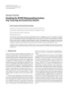
Hindawi Publishing Corporation EURASIP Journal on Advances in Signal Processing Volume 2011, Article ID 434378, 18 pages doi:10.1155/2011/434378 Research Article Feedback Amplitude Modulation Synthesis Jari Kleimola,1 Victor Lazzarini,2 Vesa V¨ lim¨ ki,1 and Joseph Timoney2 aa 1 Department of Signal Processing and Acoustics, Aalto University School of Electrical Engineering, P.O. Box 13000, 00076 AALTO, Espoo, Finland 2 Sound and Digital Music Technology Group, National University of Ireland, Maynooth, Co. Kildare, Ireland Correspondence should be addressed to Jari Kleimola, jari.kleimola@tkk.ﬁ Received 15 September 2010; Accepted 20 December 2010 Academic Editor: Federico Fontana Copyright © 2011 Jari Kleimola et al. This is an open access article distributed under the Creative Commons Attribution License, which permits unrestricted use, distribution, and reproduction in any medium, provided the original work is properly cited. A recently rediscovered sound synthesis method, which is based on feedback amplitude modulation (FBAM), is investigated. The FBAM system is interpreted as a periodically linear time-varying digital ﬁlter, and its stability, aliasing, and scaling properties are considered. Several novel variations of the basic system are derived and analyzed. Separation of the input and the modulation signals in FBAM structures is proposed which helps to create modular sound synthesis and digital audio eﬀects applications. The FBAM is shown to be a powerful and versatile sound synthesis principle, which has similarities to the established distortion synthesis methods, but which is also essentially diﬀerent from them. 1. Introduction For sinusoidal inputs, both techniques will produce a limited set of partials. In order to develop them into a useful Amplitude modulation (AM) is a well-described technique method of synthesis, one may either employ a component- of sound processing [1]. It is based on the audio-range rich carrier, or by means of feedback, add partials to modulation of the amplitude of a carrier signal generator the modulator [2]. The second option has the advantage by another signal. For each component in the two input of providing a rich output simply using two sinusoidal signals, three components will be produced at the output: the oscillators. Note that in this case only the AM method is sum and diﬀerence between the two, plus the carrier signal practical, since feedback RM produces only silence after the component. The amplitude of the output signal sAM (n) is modulator signal becomes zero. oﬀset by the carrier amplitude a, that is, The feedback AM (FBAM) oscillator ﬁrst appeared in the literature as instrument 1 in example no. 510 from sc (n) sAM (n) = [sm (n) + a] Risset’s catalogue of computer synthesized sounds [3] and , (1) a subsequently in a conference paper by Layzer [4] to whom Risset had attributed the idea. Also, a further implementation where sc (n) and sm (n) are the carrier and modulation signals, of the algorithm is found in [5]. respectively, and a is the maximum absolute amplitude of the However, the FBAM algorithm remains relatively un- carrier signal. known and, apart from the prior work cited above, is largely AM has a sister technique, ring modulation (RM) [1], unexplored. The authors started examining it in [2] and will which is very similar, but with one important diﬀerence: now expand this work in order to provide a framework for there is no oﬀset in the output amplitude, and the output a general theory of feedback synthesis by exploring the peri- signal can be expressed as odically linear time-variant (PLTV) ﬁlter theory in synthesis contexts. A further goal is to gain a better understanding sRM (n) = sm (n)sc (n). (2) of FBAM for practical implementation purposes. The novel Thus, the spectrum of ring modulation will not contain the work comprises (i) the PLTV ﬁlter interpretation of the carrier signal. method, (ii) stability, aliasing, and scaling considerations,
2 EURASIP Journal on Advances in Signal Processing which leads to the conclusion that the resulting spectrum is Amp composed of various harmonics of the fundamental f0 . In fact, as can be seen in Figure 2, a smooth pulse-like waveform + Frequency that reaches its steady-state condition within the ﬁrst period of the waveform is obtained (the reduced initial peak of the waveform is not present if the cos(·) term of (3) is replaced by a sin(·) term. The cosine form, however, simpliﬁes the theoretical discussion). Rewriting (4) as ∞ pk y (n) = (5) 2k k=0 with Figure 1: Feedback AM oscillator [4]. k pk = 2k cos[ω0 (n − m)], (6) m=0 (iii) detailed analysis of the variations, (iv) additional one gets a glimpse of what the resulting spectrum might look variations and implementations (generalized coeﬃcient- like. The products pk for k = 0 · · · 4 are the following: modulated IIR ﬁlter, adaptive FBAM, Csound opcode), and p0 = cos(ω0 n), (v) evaluation and applications of the FBAM method. The paper is organized as follows. Section 2 presents the 1 basic FBAM structure and contextualizes it as a coeﬃcient- p1 = cos(ω0 ) + cos 2ω0 n − , 2 modulated ﬁrst-order feedback ﬁlter. Section 3 proposes six general variations on the basic equation, while Section 4 p2 = cos[ω0 (n − 3)] + 2 cos(ω0 ) cos(ω0 n) + cos[3ω0 (n − 1)], explores the implementation aspects of FBAM in the form of 3 synthesis operator structures. Section 5 evaluates the FBAM p3 = 1 + cos(2ω0 ) + cos(4ω0 ) + cos 2ω0 n − 2 method against established nonlinear distortion techniques, Section 6 discusses its applications in various areas of + cos[2ω0 (n − 2)] + cos[2ω0 (n − 1)] + cos(2ω0 n) digital sound generation and eﬀects, and, ﬁnally, Section 7 concludes. 3 + cos 4ω0 n − , 2 2. Feedback AM Oscillator p4 = cos[ω0 (n − 8)] + cos[ω0 (n − 6)] + cos[ω0 (n − 2)] The signal ﬂowchart of Layzer’s feedback AM instrument is + 2 cos(4ω0 ) cos(ω0 n) + 2 cos(2ω0 ) cos(ω0 n) shown in Figure 1. This instrument is now investigated in 10 8 detail by interpreting it as a periodically linear time-variant + cos 3ω0 n − + cos 3ω0 n − ﬁlter. The basic FBAM equation with feedback amount 3 3 control is then introduced, and its impact on the stability, 4 + cos[3ω0 (n − 2)] + cos 3ω0 n − aliasing, and scaling properties of the system is discussed. 3 3 2.1. The FBAM Algorithm. First, consider the simplest FBAM + cos 3ω0 n − + cos[5ω0 (n − 2)]. 2 form, utilizing a unit delay feedback, that can be written as (7) y (n) = cos(ω0 n) 1 + y (n − 1) (3) So, for this partial sum, the fundamental (harmonic 1) is a combination of cosines having slightly diﬀerent phases and with the fundamental frequency f0 , the sampling rate fs , and amplitudes ω0 = 2π f0 / fs . The initial condition y (n) = 0, for n ≤ 0, is used in this and all other recursive equations in this paper. 1 {cos[ω0 (n − 8)] + cos[ω0 (n − 6)] This feedback expression can be expanded into an inﬁnite 16 sum of products given by 1 + cos[ω0 (n − 2)]} + cos[ω0 (n − 3)] y (n) = cos(ω0 n) + cos(ω0 n) cos(ω0 [n − 1]) 4 1 1 + cos(ω0 n) cos(ω0 [n − 1]) cos(ω0 [n − 2]) + · · · cos(ω0 ) + [cos(4ω0 ) + cos(2ω0 )] + 1 cos(ω0 n). + 2 8 ∞ (8) k = cos[ω0 (n − m)], This indicates that the harmonic amplitudes will be depen- k=0 m=0 dent on the fundamental frequency (given the various cos(·) (4)
EURASIP Journal on Advances in Signal Processing 3 this system has a periodically time-varying impulse response. 1 Secondly, the ﬁlter’s spectral properties are on their own 0.5 functions of the discrete time: at each time sample, the ﬁlter Level 0 transforms the input into an output signal depending on −0.5 the coeﬃcient values at that and preceding time instants. These types of ﬁlters were thoroughly investigated in [6, 7]. −1 Equation (11) of [6] deﬁnes a nonrecursive PLTV ﬁlter as 0 50 100 150 200 250 300 350 400 Time (samples) N y (n) = bk (n)x(n − k). (a) (11) k=0 0 Magnitude (dB) −20 The time-varying impulse response of a PLTV ﬁlter is deﬁned −40 in [6] as the output y (n) measured at time n in response to a discrete-time impulse x(m) = δ (m) applied at time m, and is −60 given for the PLTV ﬁlter of (11) by (Equation (12) of [6]) −80 −100 N 0 5 10 15 20 h(m, n) = bk (n)δ (n − k − m). (12) Frequency (kHz) k=0 (b) Consequently, the ﬁlter’s generalized transfer function (GTF) and generalized frequency response (GFR) [6, 7], which are Figure 2: Peak-normalized FBAM waveform ( f0 = 500 Hz) and its the generalizations of the transfer function and frequency spectrum. The sample rate fs = 44.1 kHz is used in this and all responses to the time-varying case, can be represented, other examples in this paper unless noted otherwise. respectively, as (Equations (2.14), (4.4), and (4.5) of [7]) ∞ N N bk (n)δ (n − k − m)zm−n = bk (n)z−k , terms in the scaling of some components). The combined H ( z , n) = magnitudes of the components will also depend on the m=−∞ k=0 k=0 fundamental frequency and sampling rate because of the N mixture of various delayed terms. bk (n)e− jkω . H ( ω , n) = Figure 2 shows that the spectrum has a low-pass shape k=0 and that the components fall gradually. Disregarding the (13) frequency dependency, a spectrum falling with a 2−k decay The case of recursive PLTV ﬁlters, such as the one (with k taken as harmonic number) can be predicted. represented by FBAM, is more involved. The time-varying However, given that there is a substantial dependency on impulse response for the ﬁrst-order recursive PLTV of (9) is the fundamental, the spectral decay will be less accented. given in [7] as Figure 2 shows also that the FBAM waveform contains a ⎧n signiﬁcant DC component. By expanding (6) further, the ⎪ g (n) ⎪ static component is observed to be generated by the odd- ⎪ a(i) = ⎪ m < n, , ⎪ ⎪i=m+1 g (m) ⎪ order products of the summation. ⎪ ⎪ ⎨ m = n, Given the complexity of the product in (4), there is little 1, h(m, n) = ⎪ (14) more to be gained, as far as the spectral description of the ⎪ ⎪0, ⎪ ⎪ m > n, ⎪ sound is concerned, proceeding this way. We will instead turn ⎪ ⎪ ⎪ ⎩ to an alternative description of the problem, studying it as an n < 0, 0, IIR system. with 2.2. Filter Interpretation. The FBAM algorithm can be inter- n preted as a coeﬃcient-modulated one-pole IIR ﬁlter that is g (n) = for n ≥ 1, g (0) = 1. a(i) (15) i=1 fed with a sinusoid. Rewriting (3) as The GTF of this ﬁlter is then deﬁned as y (n) = x(n) + a(n) y (n − 1) (9) N −1 −k k=0 h(n − k , n)z H ( z , n) = , (16) with −N 1 − g (N )z where N is the period in samples of the modulator signal x(n) = a(n) = cos(ω0 n) (10) a(n). With this in hand, the time-varying frequency response of the ﬁlter in (9) can now be written as results in a ﬁlter description for the algorithm, a periodically linear time-varying (PLTV) ﬁlter. This is a diﬀerent system N −1 − jkω k=0 h(n − k , n)e from the usual linear time-invariant (LTI) ﬁlters with static H ( ω , n) = . (17) − jNω 1 − g (N )e coeﬃcients. Firstly, instead of a single ﬁxed impulse response,
4 EURASIP Journal on Advances in Signal Processing In the speciﬁc case of FBAM, (10) tells that the modulator 1 signal a(n) is a cosine wave with frequency ω0 = 2π f0 / fs and 0.8 0.6 period in samples T0 = 2π/ω0 . In this case, to calculate the Level 0.4 GTF for this ﬁlter, we can set N = T0 + 0.5 , where · is the 0.2 ﬂoor function. Then, (17), (14), and (15) yield 0 −0.2 N −1 − jkω k=1 bk (n)e 1+ 0 50 100 150 200 250 300 350 400 450 500 H ( ω , n) = , (18) 1 − aN e− jNω Time (samples) with the coeﬃcients bk and aN set to Figure 3: Plots of the FBAM waveform (dots) and the output of its equivalent time-varying ﬁlter of (20) (solid), when fed with a k sinusoid ( f0 = 441 Hz). bk ( n ) = cos(ω0 [n − m + 1]), m=1 (19) N 1 aN = cos(ω0 m). 0.8 m=1 0.6 Level 0.4 The ﬁlter deﬁned by (9) and (10) is therefore equivalent to 0.2 a ﬁlter of length N , made up of a cascade of a time-varying 0 FIR ﬁlter of order N − 1 and coeﬃcients bk (n), and an IIR −0.2 0 50 100 150 200 250 300 350 400 450 500 (comb) ﬁlter with a ﬁxed coeﬃcient aN . The equivalent ﬁlter Time (samples) equation is, thus, Figure 4: Plot of the reconstructed FBAM signal (solid) against N −1 the actual FBAM waveform (dots), with f0 = 441 Hz. The y (n) = x(n) + bk (n)x(n − k) + aN y (n − N ). (20) reconstruction is based on the steady-state spectrum and thus does k=1 not include the transient eﬀect seen at the start of the FBAM The recursive section does not have a signiﬁcant eﬀect on the waveform. FBAM signal, as the magnitude response peaks will line up with the harmonics of the fundamental. It will, however, have implications for the stability of the ﬁlter as will be seen later. 2.3. The Basic FBAM Equation. To make the algorithm The time-varying FIR section of this equivalent ﬁlter is then more ﬂexible, some means of controlling the amount of responsible for the generation of harmonic partials and the modulation (and therefore, distortion) is inserted into the overall spectral envelope of the signal. In [7], these partials system. This can be eﬀected by introducing a modulation are called combinational components, which are added to the index β into (3), which yields output in addition to the input signal spectral components (which in the case of FBAM are limited to a single sinusoid). y (n) = cos(ω0 n) 1 + βy (n − 1) . (23) Plots of the output of this ﬁlter when fed with a sinusoid with radian frequency ω0 = 2π f0 / fs and its equivalent FBAM signal are shown in Figure 3. The ﬂowchart of this equation is shown in Figure 5. By Studies have shown that modulation of IIR ﬁlter coef- varying the parameter β, it is possible to produce dynamic ﬁcients (such as the coeﬃcient-modulated allpass) has spectra, from a pure sinusoid to a fully-modulated signal a phase-distortion eﬀect on the input signal [8–10]. In with various harmonics. The action of this parameter is addition, the amplitude modulation eﬀect caused by the demonstrated in Figure 6, which shows the spectrogram of time-varying magnitude response will help in shaping the a FBAM signal with β sweeping linearly from 0 to 1.5. The output signal. To demonstrate this, the FBAM signal can signal bandwidth and the amplitude of each partial increase be reconstituted using phase and amplitude modulation, with the β parameter. Notice that this is a simpler relation deﬁned by than in frequency modulation (FM) synthesis [11], in which partials are momentarily faded out as the modulation index y (n) = A(n) cos ω0 n + φ(n) , (21) is changed (see, e.g., Figure 4.2 on page 301 in [12]). The maximum value of β will mostly depend on the where tolerable aliasing levels, as higher values of β will increase A(n) = |H (ω0 , n)|, φ(n) = arg(H (ω0 , n)), (22) the signal bandwidth signiﬁcantly. Even higher values of this parameter will also cause stability problems, which are with H (ω, n) deﬁned by (18) and setting ω = ω0 . A plot discussed below. of this reconstruction and its equivalent FBAM waveform is shown on Figure 4, where the steady-state signals are seen to match each other. It is worth pointing out that this result 2.4. Stability and Aliasing. The stability of time-varying ﬁlters is generally diﬃcult to guarantee [13]. However, in can be alternatively inferred from the similarities between the periodic time-varying ﬁlter transfer function and the the present case, it is possible to have a stable algorithm by expansion of the FBAM expression in (4). controlling the amount of feedback in the system. From (20)
EURASIP Journal on Advances in Signal Processing 5 cos(ω0 n) 2 Out 1.8 1.6 1.4 z −1 1.2 β β 1 0.8 0.6 Figure 5: Flowchart of the basic FBAM equation, where z−1 denotes 0.4 the delay of a unit sample period. 0.2 0 500 1000 1500 2000 2500 3000 3500 4000 10 Frequency (Hz, 88-key piano range) 0 Figure 7: Stability (dashed) and aliasing (solid: fs = 44.1 kHz, −12 dotted: fs = 88.2 kHz) limits of FBAM. 8 −24 Frequency (kHz) −36 1 6 0.5 −48 Level 0 4 −60 −0.5 −72 −1 2 0 50 100 150 200 250 300 350 400 −84 Time (samples) −96 0 (a) (dB) 0 0.2 0.4 0.6 0.8 1 1.2 1.4 0 β Magnitude (dB) −20 Figure 6: Spectrogram of the FBAM output with β varying from 0 −40 to 1.5 ( f0 = 500 Hz). −60 −80 −100 and (23), the impulse response of the system is noted to 0 5 10 15 20 decrease in time when Frequency (kHz) (b) β aN < 1, (24) Figure 8: FBAM spectrum and waveform with β = 1.9 ( f0 = that is, when the product of instantaneous coeﬃcient values 500 Hz). over the period multiplied by the modulation index β is less than unity [7]. The dashed line of Figure 7 plots the maximum β values satisfying this stability condition, obtained through iterated spectral analysis: the frequency showing that the stability is frequency dependent. The axis was sampled at 100 points, and for each fundamental approximate stability limit is given by βstable ≈ 1.9986 − 0. frequency, the β value was increased until the magnitude 00003532 ( f0 − 27.5). of the strongest aliasing harmonic reached the −80 dB limit In practice, however, the system stability will never (the algorithm is available at [15]). The solid curve ( fs = become the limiting issue. This is because for values of β well 44.1 kHz) shows that for fundamental frequencies lower within the range of stable values, an objectionable amount of than 1300 Hz, when the curve is smooth, the maximum aliasing is obtained. So, in fact, the real question is how large usable β values are determined by the overmodulation can the modulation index be before the digital baseband is foldover distortion discussed above. For higher fundamental exceeded. This will of course depend on the combination frequencies, the stepwise shape of the curve suggests that the of the sampling rate and fundamental frequency. Taking for −80 dB limit is determined by the harmonics folding back instance f0 = 500 Hz and fs = 44100 Hz, one observes to the digital baseband at the Nyquist limit. The dotted curve that for β = 1.9, there is considerable foldover distortion ( fs = 88.2 kHz) shows that oversampling increases the usable throughout the spectrum (see Figure 8). The distortion is β range by stretching the maximum β values towards higher also visible in the signal waveform as the formation of wave frequencies relative to the oversampling amount. packets similar to those found in overmodulated feedback FM synthesis [14]. The solid and dotted curves in Figure 7 show the 2.5. Scaling. The gain of the FBAM system varies consid- erably with diﬀerent β values—in a frequency-dependent maximum β values that keep the amount of aliasing 80 dB manner—and grows rapidly after β exceeds unity. This below the loudest harmonic (the fundamental) at sample rates of 44.1 kHz and 88.2 kHz, respectively. The curves were makes the output gain normalization a challenge, which
6 EURASIP Journal on Advances in Signal Processing will examine a number of these (see Figure 10), starting from 0 the insertion of a feedforward term, which can subsequently be used for an allpass ﬁlter-derived structure, and proceeding to heterodyning, nonlinear distortion, nonunitary delays, and the generalization of FBAM as a coeﬃcient-modulated −6 Magnitude (dB) ﬁlter. 3.1. Variation 1: Feedforward Delay. A simple way of gener- −12 ating a diﬀerent waveshape is to include a feedforward delay term in the basic FBAM equation (see Figure 10(a)) y (n) = cos[ω0 (n − 1)] − cos(ω0 n) 1 + βy (n − 1) . (25) −18 In this case, besides the DC oﬀset, there is no change in the spectrum as the feedforward delay will not change the shape 500 1000 1500 2000 2500 3000 3500 4000 of the input (i.e., it remains a sinusoid). However, because Frequency (Hz, 88-key piano range) of the half-sample delay caused by the feedforward section, Figure 9: FBAM gain (solid) and its polynomial approximation the shape of the waveform is diﬀerent, as its harmonics are (dotted). β = 0.1 (bottom)· · · β = 0.9 (top). given diﬀerent phase oﬀsets. Figure 11 shows the waveform and spectrum of this FBAM variant. can, however, be resolved by approximate peak-scaling and 3.2. Variation 2: Coeﬃcient-Modulated Allpass Filter. From average power balancing algorithms. the feedforward delay variation discussed above, it is possible Figure 9 shows that the peak gain of the basic FBAM to derive a variant that is similar to the coeﬃcient-modulated equation (solid line) can be approximated well within a 1- allpass ﬁlter described in [8] and used for phase distortion dB deviation by polynomials of degree 1 (β < 0.7) and of synthesis in [9, 10]. The general form of this ﬁlter is degrees 2, 3, and 5 (corresponding to β values 0.7, 0.8, and 0.9, resp.). y (n) = x(n − 1) − a(n) x(n) − y (n − 1) . (26) The scaling factors for in-between β values can be found by linear interpolation, provided that the polynomial This is translated into the presented FBAM form by equating approximations are taken at suﬃciently small intervals (e.g., a(n) to the input signal x(n) = cos(ω0 n), as in Section 2.1 setting Δβ = 0.05 generated acceptable results). Scaling factors for β ≥ 1 follow power-law approximations, which y (n) = cos[ω0 (n − 1)] − β cos(ω0 n) cos(ω0 n) − y (n − 1) . are problematic with low fundamental frequencies where the (27) FBAM gain rate changes most rapidly. A two-dimensional The ﬂowchart of the coeﬃcient-modulated allpass ﬁlter is lookup table (Δβ = 0.05, 100 frequency samples) with shown in Figure 10(b), while its waveform and spectrum are bilinear interpolation was found to be able to provide more plotted in Figure 12. accurate results across the entire stable β range. Each entry in The resulting process is equivalent to a form of phase the table can be precalculated by evaluating one half period modulation synthesis, as discussed in [9]. As with the basic of (23) using a sine input and ﬁnding the maximum value of the result. The lookup table and the function coeﬃcients version of FBAM, it is possible to raise the modulation index β above one, as this variant exhibits similar stability and are available at [15]. The two-dimensional lookup table aliasing behavior. approach was observed to provide transient-free scaling for control rate parameter sweeps. Equation (23) may alternatively be evaluated at the 3.3. Variation 3: Heterodyning. Employing a second sinu- control rate for each block of output samples. Another online soidal oscillator as a ring-modulator provides a further solution is to use a root-mean-square (RMS) balancer [1] variant to the basic FBAM method. This heterodyning that consists of two RMS estimators and an adaptive gain variant can have two forms, by placing the modulator inside control. The FBAM output and cosine comparator signals are or outside the feedback loop, as shown in Figures 10(c) and ﬁrst fed into the RMS estimators, which rectify and low-pass 10(d), respectively, producing diﬀerent output spectra. ﬁlter their inputs to obtain the estimates. The scaling factor is then calculated from a ratio of the two RMS estimates. This 3.3.1. Type I: Modulator inside the Feedback Loop. In this solution is suﬃciently general to work with the variations structure, the basic FBAM expression is simply multiplied by discussed in the next section. a cosine wave of a diﬀerent frequency y (n) = cos(θn) cos(ω0 n) 1 + βy (n − 1) , (28) 3. Variations where θ is the normalized radian frequency of the ring- The basic structure of FBAM provides an interesting plat- form on which new variants can be constructed. This section modulator. The main characteristic of this variant is that the
EURASIP Journal on Advances in Signal Processing 7 z −1 z −1 β + cos(ω0 n) Out + − cos(ω0 n) Out − z −1 z −1 β + − (a) (b) cos(θn) cos(θn) cos(ω0 n) cos(ω0 n) Out Out z −1 z −1 β β (c) (d) cos(ω0 n) cos(ω0 n) Out Out z −1 z −D β β f (·) (e) (f) Figure 10: FBAM variation ﬂowcharts. The z−1 and z−D symbols denote delays of one and D sample periods, respectively. 1 1 0.5 0.5 Level Level 0 0 −0.5 −0.5 −1 −1 0 50 100 150 200 250 300 350 400 0 50 100 150 200 250 300 350 400 Time (samples) Time (samples) (a) (a) 0 0 Magnitude (dB) Magnitude (dB) −20 −20 −40 −40 −60 −60 −80 −80 −100 −100 0 5 10 15 20 0 5 10 15 20 Frequency (kHz) Frequency (kHz) (b) (b) Figure 12: Waveform and spectrum of FBAM variation 2 (β = 1, Figure 11: Waveform and spectrum of FBAM variation 1 (β = 1, f0 = 500 Hz), see Figure 10(b). f0 = 500 Hz), see Figure 10(a). whole of the modulated signal is fed back to modulate the spectrum. This ratio also determines the general shape of amplitude of the ﬁrst oscillator, as shown in Figure 10(c). the spectrum, which exhibits regularly-spaced peaks. Both In general, if the ratio of frequencies of the modulator and the fundamental frequency and the spacing of peaks are FBAM oscillators is of small integers, the result is a harmonic dependent on this frequency ratio.
8 EURASIP Journal on Advances in Signal Processing 1 1 0.5 0.5 Level Level 0 0 −0.5 −0.5 −1 −1 0 50 100 150 200 250 300 350 400 0 50 100 150 200 250 300 350 400 Time (samples) Time (samples) (a) (a) 0 0 Magnitude (dB) Magnitude (dB) −20 −20 −40 −40 −60 −60 −80 −80 −100 0 5 10 15 20 −100 0 5 10 15 20 Frequency (kHz) Frequency (kHz) (b) (b) Figure 14: Heterodyne FBAM variation 3-II ( f0 = 500 Hz, β = 0.3, Figure 13: Heterodyne FBAM variation 3-I ( f0 = 500 Hz, β = 0.2, cosine carrier frequency 4000 Hz (8 : 1 ratio)), see Figure 10(d). modulator frequency 4000 Hz (8 : 1 ratio)), see Figure 10(c). multiple of the FBAM f0 . Figure 14 depicts the waveform In some cases, harmonics are missing or they have very and spectrum of (29), with k = 8 (β = 0.3, f0 = 500 Hz, small amplitudes, such as in the case of the 8 : 1 ratio shown and fs = 44100 Hz). Note that the bandwidth of the resonant in Figure 13. Here, harmonics 1, 3, 6, 8, 10, 13, 15, 17, 19, region is proportional to β and that the practical β range is 22, 24, 26, and so forth are seen to be missing (or have an amplitude at least −100 dB from the maximum). The considerably wider than in heterodyning type I. A more general algorithm for formant synthesis would peaks in the spectrum are around harmonics 8 (missing), 16, require the use of two carriers tuned to adjacent harmonics 24 (missing), 32 and 40 (missing). This method provides a around the resonance frequency fc , whose signals are rich source of spectra. However, its mathematical description weighted and mixed together to provide the output is very complex and the matching of parameters to the spectrum is not as straightforward as in other variants. On fc the plus side, the β parameter (FBAM modulation index) k = int , (30) maps simply to spectral richness and it does not have a major f0 eﬀect on the relative amplitude of harmonics (beyond that fc of adding more energy to higher components). However, g= − k, (31) f0 because of aliasing issues, the practical β range decreases rapidly with increasing θ/ω0 ratios. y (n) = cos(ω0 n) 1 + βy (n − 1) , (32) 3.3.2. Type II: Modulator outside the Feedback Loop. The s(n) = y (n) 1 − g cos(kω0 n) + g cos[(k + 1)ω0 n] . second form of heterodyne FBAM places the modulation This structure can be used for eﬃcient synthesis of res- outside the feedback loop (see Figure 10(d)). In other words, the basic FBAM algorithm is used to create a modulator onances from vocal formants to emulation of analogue signal with a baseband spectrum, which is then shifted to be synthesizer sounds. centered on the cosine carrier frequency θ , as deﬁned by the following pair of equations: 3.4. Variation 4: Nonlinear Waveshaping. An interesting modiﬁcation of the FBAM algorithm can be implemented y (n) = cos(ω0 n) 1 + βy (n − 1) , by employing a nonlinear mapping of the feedback path, (29) s(n) = cos(θn) y (n). a process commonly known as waveshaping [20, 21]. The general form of the algorithm is A similar structure is seen in the double-sided Discrete Sum- y (n) = cos(ω0 n) 1 + f β y (n − 1) , mation Formula (DSF) algorithm [16], as well as in Phase- (33) Aligned Formant (PAF) synthesis [17] (which is derived from where f (·) is an arbitrary nonlinear waveshaper DSF) and phase-synchronous Modiﬁed FM [18, 19]. This heterodyne principle is very useful for generating resonant (Figure 10(e)). There are a variety of possible transfer spectra and formants by setting θ = kω0 , with k > 0 functions that may be employed for this purpose. The most useful ones appear to be trigonometric (sin(·), cos(·), etc.) and an integer, that is, making the cosine frequency a
EURASIP Journal on Advances in Signal Processing 9 1 1 0.5 0.5 Level Level 0 0 −0.5 −0.5 −1 −1 0 50 100 150 200 250 300 350 400 0 50 100 150 200 250 300 350 400 Time (samples) Time (samples) (a) (a) 0 0 Magnitude (dB) Magnitude (dB) −20 −20 −40 −40 −60 −60 −80 −80 −100 −100 0 5 10 15 20 0 5 10 15 20 Frequency (kHz) Frequency (kHz) (b) (b) Figure 15: FBAM variation 4 with cosine waveshaping (β = 1, f0 = Figure 16: FBAM variation 4 with ABS waveshaping (β = 1, f0 = 500 Hz), see Figure 10(e). The transient appears because the initial 500 Hz), see Figure 10(e). state of the ﬁlter was not set up appropriately. As can be seen, this expression only diﬀers from feedback and a few piecewise-linear waveshapers (such as the absolute FM by the added sine and cosine components at f0 . value function ABS). Equation (37) demonstrates that it is possible to create The case of cosine and sine waveshapers is particularly transitions between cosine (and sine) waveshaped FBAM and interesting; for instance, feedback FM. This might be a useful feature to be noted in y (n) = cos(ω0 n) 1 + cos β y (n − 1) (34) implementations of the technique. Choosing the ABS transfer function provides another produces a signal that is closely related to feedback FM means of removing even harmonics from the FBAM spec- synthesis [22]. To demonstrate the similarities, start with the trum, as shown in Figure 16. This is because, like the cosine FM equation [11] waveshaper, the absolute value function is an even function. Such a waveshaper will feature only even harmonics of its y (n) = cos[ω0 n + m(n)] (35) input signal frequencies [19]. However, in the current setup, and set the modulator function m(n) = y (n − 1) to the waveshaper output is heterodyned by a cosine wave tuned implement the feedback. Expanding this gives to its fundamental frequency, thus generating odd harmonics of that frequency. y (n) = cos ω0 n + y (n − 1) Another interesting feature of the ABS waveshaper is that it maintains the relative amplitudes of odd components close = cos(ω0 n) cos y (n − 1) − sin(ω0 n) sin y (n − 1) . to the values in the basic FBAM expression. Therefore, it (36) provides an interesting means of varying odd-even balance of a synthesized tone by combining this variant with the basic So, the cosine-waveshaped FBAM partially implements the FBAM technique. feedback FM equation. As it turns out, this partial imple- The aliasing properties of variation 4 depend naturally mentation removes all even harmonics from the spectrum. This is shown in Figure 15, which illustrates also the eﬀect of on the choice of the waveshaper. For the presented cases, the practical β range is slightly more restricting than the general an improper initial state: the waveform contains a transient, case shown in Figure 7. which is due to a poorly chosen initial feedback state value. Here, y (0) = 1 instead of the recommended peak value of the steady-state waveform. 3.5. Variation 5: Nonunitary Feedback Periods. The early It is possible to closely approximate feedback FM by works on feedback amplitude modulation utilized various combining two sinusoidal waveshaper FBAM structures, one feedback delay lengths. In [3], Risset does not discuss the of them using cosine and the other sine functions design in detail, but from his MUSIC V code the feedback delay is seen to be one sample block (existing FORTRAN y (n) = cos(ω0 n) 1 + cos β y (n − 1) code shows that the program processes the signal on a block-by-block basis [23]). Layzer’s article [4] describes the − sin(ω0 n) 1 + sin β y (n − 1) (37) algorithm as based on a ﬁxed feedback delay of 512 samples = cos ω0 n + βy (n − 1) + cos(ω0 n) − sin(ω0 n). (the system block size). A footnote mentions an alternative
10 EURASIP Journal on Advances in Signal Processing implementation by F.R. Moore allowing delays from one to 1 512 samples. In [5], the feedback delay is equivalent to the 0.5 Level default processing block size for the system in which it is 0 implemented (64 samples). The diﬀerences in feedback delay −0.5 lengths are important to the resulting output. −1 The feedback delay of the basic FBAM can be generalized 4410 4510 4610 4710 4810 4910 to allow for an arbitrary period size (see Figure 10(f)). Time (samples) Instead of limiting the delay to one sample, it can be made (a) variable 0 Magnitude (dB) y (n) = cos(ω0 n) 1 + βy (n − D) , −20 (38) −40 −60 where D is the delay length in samples. From a ﬁlter −80 perspective, this equation deﬁnes a coeﬃcient-modulated −100 comb ﬁlter (which is fed a cosine wave as input). As such 0 5 10 15 20 the delay D can be expected to have an eﬀect on the Frequency (kHz) output spectrum. Diﬀerent waveshapes can be produced (b) with various delays, but the spectrum will be invariant if the ratio of the delay time TD = fs /D and the modulation Figure 17: FBAM variation 5 (β = 0.85, f0 = 441 Hz) with feedback frequency, which is in this case also f0 , is preserved. For this period D = 100 (solid), see Figure 10(f). The dashed line plots the to be eﬀective, the delay time will be inversely proportional to basic FBAM with period D = 1. the change in fundamental frequency. This principle should additionally allow keeping the basic FBAM spectrum f0 - To gain an understanding of the type of spectra obtained, invariant by lengthening the delay as frequency decreases. Of (40) can be partially evaluated limiting k to 4 course, there will be an upward limit of one-sample delay (if fractional delays are not desired). 4 βk−1 cos (ω0 n)k An interesting case arises when the TD : f0 ratio is one, − and so D = 2πω0 1 = fs / f0 . In this case, the FBAM expression k=1 becomes much simpler β − β3 1 3 3 β + β3 + 1 + β2 cos(ω0 n) + = cos(2ω0 n) 2 8 4 2 2π y (n) = cos(ω0 n) 1 + βy n − ω0 1 1 + β2 cos(3ω0 n) + β3 cos(4ω0 n). 4 8 ∞ k (41) βk = cos(ω0 n − 2πm) (39) m=0 k=0 In order to obtain a continuous range of delay times, ∞ some form of interpolation is required. As observed in [24], cos(ω0 n) βk−1 cos (ω0 n)k = = this will have an eﬀect on the output. Although it is beyond , 1 − β cos(ω0 n) k=1 the scope of the present study to discuss the best interpola- tion methods for fractional delay FBAM, good results have for 0 ≤ β < 1 (see Figure 17); with β = 1, there is a singularity been observed with a linear interpolation method in delays at cos(0), and with β > 1, the series is divergent and the longer than a few samples. For very short delays, a higher closed form does not apply. It is also possible to expand the precision interpolator would most likely be required. summation in (39) to obtain its spectra The aliasing properties of variation 5 follow closely the general case of Figure 7. However, we observed that the ∞ system becomes unstable with large β values when D = fs / f0 βk−1 cos (ω0 n)k or D = fs / 2 f0 . k=1 ∞ 3.6. Variation 6: Coeﬃcient-Modulated First-Order IIR Filter. β2k−1 cos (ω0 n)2k + β2k−2 cos (ω0 n)2k−1 = So far, the focus has been on self-modulation scenarios that k=1 share a single sinusoid between the carrier and the modu- ⎧ ⎫ ⎛⎞ ⎛ ⎞ ⎨ 1 2k ⎬ ∞ k−1 lating signal. The FBAM algorithm is now generalized as a 2k ⎝ ⎠+ 2 ⎝ ⎠ cos[(2k − 2m)ω0 n] 2k−1 = coeﬃcient-modulated IIR ﬁlter by relaxing the constraint of β ⎩ 22k m ⎭ 22k m m=0 k=1 (10) and decoupling the input signals, that is, the carrier x(n) ⎛ ⎞ and the modulator m(n), into independent and arbitrary k−1 2k − 1 2β2k−2 ⎝ ⎠ cos[(2k − 2m − 1)ω0 n]. inputs as shown in Figure 18. Rephrasing (23) as + 2k−1 2 m m=0 y (n) = x(n) + m(n)βy (n − 1) (42) (40)
EURASIP Journal on Advances in Signal Processing 11 x(n) Table 1: FBAM input signals and synthesis parameters. Out Input Category Variation Description z−1 x(n) Signal Common Carrier β m(n) Signal Common Modulator m(n) r (n) Signal 3 Ring modulator Figure 18: FBAM variation 6 with decoupled input signals. v Parameter Common Variation number β Parameter Common Feedback amount ws Parameter 4 Waveshaper type oﬀers two additional degrees of freedom, because the D Parameter 5 Feedback delay length frequencies and the waveforms of both input signals can now be chosen independently. In the present study, the modulator signal should be periodic, however. sizes, which would allow diﬀerent spectral characteristics at For sinusoidal carrier and modulator signals with β = 0, the output (and of course, in this case, we are no more strictly the spectrum of (42) consists of a single component that speaking of a ﬁrst-order ﬁlter structure). is located at the carrier frequency fx . As β is increased, The stability of the ﬁrst method depends on the input the component at fx is skirted with upper and lower signal matching the conditions set by (24). A special case sidebands and the resultant spectra will gradually grow might occur when the input signal is not periodic, in into the formant-shaped structure shown in Figure 14. The which case the PLTV ﬁlter theory does not apply. The spectral structure of the formant can be controlled by the second method follows the stability condition as studied in modulation frequency fm , as the sideband components will Section 2.4. The aliasing properties depend largely on the appear at frequencies fx ± k fm . Negative frequencies alias input waveform. at DC back to the positive domain, and, as discussed in Section 3.3, frequency ratios fx : fm of small integers will 4. Implementations generate harmonic spectra, while more complex ratios result in inharmonic timbres. This section reﬁnes the FBAM operator and algorithm A complex periodic modulation signal generates upper concepts introduced in [2] and discusses their implemen- and lower sidebands for each of its spectral component, tation in two popular audio synthesis environments. These which happens also in complex modulator FM [25, 26]. The concepts are related to their FM synthesis counterparts sidebands consist of partials that are located at frequencies described in [28]. ±k fx around the original modulator component, and, therefore, the spectral structure of the formants can be 4.1. FBAM Operator. The audio rate interface of the FBAM controlled by the carrier oscillator frequency fx . ﬂowcharts depicted in Figures 5 and 10 consists of two The aliasing properties of variation 6 depend on the input (cos(ω0 n), cos(θn)), and one output (Out ) signals. frequency ratio between the carrier and the modulator. The shared cos(ω0 n) input can be further decoupled into Larger frequency ratios increase the amount of high end separate carrier and modulator signals x(n) and m(n), as spectral content, and, therefore, the risk of aliasing is bigger discussed in Section 3.6. The control rate interface of the than in the general case of fx : fm = 1. ﬂowcharts consists of the synthesis parameters. By hiding the implementation details of the variations, the FBAM system 3.6.1. Adaptive Feedback AM. The ﬁlter interpretation of can be considered as a black box that is interfaced with the FBAM allows its treatment as an adaptive audio eﬀect. This inputs listed in Table 1. The contents of the FBAM black box can be implemented in two general lines, based on how the includes a waveshaper (variation 4), a delay line (variation input signal shall be used to control the ﬁlter behavior. The 5), an output level scaling unit, and a set of state variables, ﬁrst and the simplest method is to exchange the sinusoidal multipliers, and adders for the algorithmic details, as shown signal with an arbitrary input. In this method, the ﬁlter in the FBAM ﬂowcharts. coeﬃcient will be modulated by the input Cascading a sinusoidal carrier oscillator, the FBAM black box, and an envelope-controlled gain unit brings forth the y (n) = x(n) 1 + βy (n − 1) . (43) Feedback AM Operator shown in Figure 19. The signal inputs r (n) and m(n) can be derived from the outputs of other The second alternative implementation, based on (42) and FBAM operators or from the carrier oscillator output x(n) following the principles adopted in Adaptive FM [27], uses a by means of the modulation source selector SM . pitch tracking algorithm to control the modulator frequency. In addition, the value of β can be made proportional To simplify the tuning of the system, the fundamental to the amplitude of the input signal with the use of an frequency of the carrier oscillator is parametrized as a vector [osc] = ( fB , q), where fB is the base frequency envelope follower. This method is perhaps more ﬂexible as one can avail of a choice of modulator signals and a diﬀerent and q is the frequency ratio, giving f0 = q fB . The other parameter vectors are [ f bam] = (v, β, ws , D), interfacing modulator frequency (whereas the ﬁrst method locks a 1 : 1 ratio between the input and coeﬃcient modulator). In the FBAM black box, and [env] = (A, D, S, R), describing addition, both alternatives can also avail of nonunitary delay the attack/decay/sustain/release settings of the envelope
12 EURASIP Journal on Advances in Signal Processing as a Pure Data (Pd) [29] external ( f bam ∼), which is [ f bam] g equipped with three signal inlets, four parameter inlets, and one signal outlet. The external uses block-based processing, r (n) rm but supports also single-sample feedback delays by main- taining its state between successive block-based processing car AMP OSC y (n) calls. However, sample-based cross-modulation between two [osc] FBAM operators is possible only by setting Pd’s global block size to 1. mod EG The f bam ∼ external was then patched with native Pd m(n) OSC ∼, ∗ ∼, and adsr objects implementing the OSC, AMP, SM [env] and EG blocks of the operator. The patch was interfaced with inlet and outlet ports carrying the signals and synthesis Figure 19: FBAM operator, interfaced by audio rate signals (solid) parameters discussed in Section 4.1 and encapsulated as and control rate parameters (dashed). the f bamOP Pd abstraction, which ﬁnally implements the FBAM operator. Table 2: Computational load of FBAM, its variations, and related synthesis methods. 4.4. Csound Opcode. In Csound [30], we propose a simple user-deﬁned opcode (UDO) implementing the coeﬃcient- Method Figure MUL ADD Scale Total TLU modulated ﬁrst-order ﬁlter, which can then be used with FBAM 5 1 1 1 3 1 a variety of inputs in the various combinations discussed Variation 1 10(a) 1 2 1 4 1 in this paper. It could alternatively be used inside another Variation 2 10(b) 1 2 1 4 1 UDO implementing a similar structure to the Pd code in the Variation 3 10(c), 10(d) 2 1 1 4 2 previous section (Figure 19). The ﬁlter UDO is isolated from Variation 4 10(e) 1 1 1 3 2 the other parts of the code for eﬃciency reasons: it requires Variation 5 10(f) 1 1 1 3 2 a processing vector of one sample for the feedback to be Variation 6 18 1 1 1 3 2 implemented. As this is computationally costly, it is separated PAF 1 0 2 3 3 from the rest of the code, as shown in Listing 1. With this in hand, the basic FBAM algorithm is imple- ModFM 2 1 1 4 3 mented with the code presented in Listing 2. DSF 5 3 1 9 2 5. Evaluation generator EG. Parameter g deﬁnes the maximum amplitude of the output y (n). It should be noted that the encapsulated This section evaluates the FBAM method by comparing it to FBAM block may be parametrized so that the output of the related nonlinear synthesis techniques. First the basic FBAM operator consists only of the carrier signal produced by the equation is contextualized in the parameter spaces of the OSC block. related techniques, and then the computational load of the methods are compared. 4.2. FBAM Algorithms. Two or more FBAM operators may be arranged into multioperator conﬁgurations called FBAM 5.1. Relation to Existing Nonlinear Distortion Methods. Equa- algorithms. Parallel multicarrier conﬁgurations simply mix tion (21) reconstructed the basic FBAM waveform using the outputs of the operators together, whereas cascaded a hybrid amplitude and phase modulation technique. By setups connect the output of the modulator operator to ignoring the phase modulation component φ(n) in (21), one the m(n) and/or r (n) inputs of the carrier. As a special can look at the eﬀect of AM separately (see Figure 21(a)). On case of the cascaded arrangement, the output of the carrier the other hand, by setting the A(n) component to unity, one operator can be fed back to the m(n) input of the modu- can see the eﬀect of the isolated phase modulation operation, lator operator, thereby producing cross-modulated timbres. as shown in Figure 21(b). As can be seen, the FBAM output is Figure 20 shows three algorithms that are used in the FBAM mostly determined by the AM operation between a complex application examples of Section 6. signal and a sinusoid and the eﬀect of phase modulation in In parallel topologies, the g parameter is utilized as a (21) is minor. balance control, whereas in cascades the g and the [env] This suggests that FBAM is more related to the ring- vector of the modulator provide dynamic control over the modulation-based PAF [17] and the recent ModFM [18, spectral richness of the carrier output. The [osc] vectors 19] methods than it is to the classic FM [11] synthesis deﬁne the frequency ratio between the modulator and the technique. Figure 22 compares the waveform and spectrum carrier, thus aﬀecting the harmonic or inharmonic structure of FBAM (dashed), PAF (solid), and ModFM (dots). The of the spectrum. parameters were chosen by ﬁrst selecting the maximum β value according to the criteria of Figure 7, then normalizing 4.3. Pure Data External and Abstraction. The FBAM black the magnitude of the fundamental to 0 dB, ﬁnding the highest frequency component above the −100 dB threshold, box was implemented in the C programming language
EURASIP Journal on Advances in Signal Processing 13 B 1 1 1 2 ext 5 1, 4 3-II 3-II 3-II 3-II Loss + + Out + Out Out (a) (b) (c) Figure 20: FBAM algorithms for (a) subtractive, (b) formant, and (c) abstract physical modeling sound synthesis arrangements. Variation numbers are given inside the operator boxes (B denotes the basic FBAM equation). and ﬁnally matching the magnitudes of the highest partials. The waveform maxima in Figure 22(a) have been time- opcode Cmf,a,aak aligned for easy comparison, showing that the waveform setksmps 1 peak is the narrowest in ModFM and widest in PAF. This ay init 0 is reﬂected in the spectrum plot of Figure 22(b), where the asig,amod,kb xin spectral slope of FBAM is less accented than the exponential = asig + amod∗ ay∗ kb ay decay of PAF, but steeper than the one produced by ModFM. xout ay The DSF formulation of PAF is similar to (4) given in endop [16]. A related closed form approximation of FBAM is given by Listing 1: Csound UDO for the coeﬃcient-modulated ﬁrst-order IIR ﬁlter. cos(ω0 n) y (n) = , (44) [1 − 2a cos(ω0 n) + a2 ]3 6. Applications The brief discussion of FBAM applications in the authors’ which is similar to Equation (593) of [31], in which the ratio earlier work is now extended, and the sonic palette of FBAM parameter a is dependent on the β and ω0 parameters of is expanded further with three novel applications. Additional FBAM. The waveform and spectrum of (44) are shown in application examples are available at the accompanying web Figures 23(a) and 23(b), while its normalized waveshaper page [15]. formulation is plotted in Figure 23(c). As expected, a waveshaper based on Chebyshev’s polyno- 6.1. Subtractive Synthesis without Resonant Filters. FBAM can mials [1] can reproduce the magnitude spectrum of FBAM exactly when β = 1. Its transfer function takes an exponential imitate classic analog waveforms with variations 1 and 4. Although the spectral brightness in these cases is limited shape with a close match to the waveshaper shown in (see Figures 11, 15, and 16), it may be conveniently shaped Figure 23(c). with the β parameter. A single FBAM operator can, therefore, function as a simple low-cost subtractive synthesizer that 5.2. Computational Load. Table 2 summarizes the number of implements both the source oscillator and the low-pass ﬁlter multiplications (MUL, Scale), additions (ADD), and table of a virtual analog system. This basic scheme can be further lookups (TLU) for the basic FBAM, its variations, and related reﬁned by simulating the resonance characteristics of the synthesis techniques per output sample. Each oscillator low-pass ﬁlter with (32). The structure of such a setup is involved in the algorithm is counted as a table-lookup shown in Figure 20(a). operation. It is noted that FBAM, PAF, and ModFM are close A related DSF-based implementation [32], without reso- to each other in the total number of simple operations, but nance control, requires 25 operations per output sample for that FBAM has the beneﬁt of not using precomputed lookup the direct closed form evaluation and additional control rate operations for dynamic cut-oﬀ frequency updates (whereas tables in the complex modulator signal evaluation. This is an advantage of FBAM, because interpolating table lookups are FBAM uses 5 operations in total). However, the spectral considerably more resource consuming than simple addition brightness of the DSF-based method is considerably higher and multiplication operations. DSF gains the widest output and, at the same time, bandlimited. FBAM can control the amount of aliasing by scaling β bandwidth at the cost of additional operations per output sample. with the curve shown in Figure 7, while the bandwidth of
14 EURASIP Journal on Advances in Signal Processing opcode Fbam,a,kkki kamp,kfreq,kbeta,itab xin asig oscili kamp,kfreq,itab aout Cmf asig,asig,kbeta xout aout endop Listing 2: Csound UDO for the basic FBAM algorithm. 1 1 0.5 Level 0.5 Level 0 −0.5 0 −1 0 50 100 150 200 250 300 0 50 100 150 200 250 Time (samples) Time (samples) (a) (a) 1 0 Magnitude (dB) 0.5 −20 Level 0 −40 −0.5 −60 −1 −80 0 2 4 6 8 10 12 0 50 100 150 200 250 300 Frequency (kHz) Time (samples) (b) (b) Figure 22: Waveform and spectrum of FBAM (β = 1.62, dashed), Figure 21: (a) FBAM waveform (dashed) and reconstructed PAF (bandwidth δ = 0.164, solid), and ModFM (k = 25, dotted). using AM (solid). (b) Cosine waveform (dashed) and FBAM Signals were generated with fc = fm = 500 Hz. reconstruction using PM (solid). Signals were generated with β = 1 and f0 = 500 Hz. FBAM can be increased by oversampling. However, a more for vocal timbres). Carrier β and g values control the width cost-eﬀective bandwidth extension is achieved by adding and relative amplitude of the formant. partials to the modulator signal, for example, by raising Figure 25 shows an example FBAM vocal timbre, with the modulator to the third power, yielding cos3 (ω0 n) = fundamental frequency f0 = 196 Hz and approximate 0.75 cos(ω0 n)+0.25 cos(3ω0 n). Figure 24 compares the wave- formants at f1 = 700 Hz, f2 = 1090 Hz, and f3 = form and spectrum of this extended bandwidth modiﬁcation 2700 Hz. Because the formant frequencies do not coincide to the basic FBAM output, using β values that keep the with the harmonic series of the fundamental, each formant aliasing level −100 dB from the maximum. Note that the is modeled using the double-carrier formula of (32). For cubed cosine modulator permits higher β values because example, formant f3 is modeled using harmonic ordinals | cos(ω0 n)| ≤ 1. The cost of this modiﬁcation is two kLO = int( f3 / f0 ) = 13 and kHI = kLO + 1 = 14, giving multiplications per output sample. fLO = 13 f0 and fHI = 14 f0 , thereby coinciding with the harmonic spectra of the fundamental f0 . The modulator is 6.2. Formants. FBAM can synthesize formant-based timbres formed as a weighted sum of two cosine oscillators, which are tuned to frequencies fLO and fHI and weighted using with parallel resonator stacks, as shown in Figure 20(b). In linear interpolation as gHI = f3 / f0 − kLO and gLO = 1 − gHI . this algorithm, each modulator operator is tuned to the center frequency of the formant, while all carriers are tuned The bandwidth of formant 3 is controlled by setting the modulation index of the carrier β3 = 0.6, and, ﬁnally, the to the fundamental frequency of the tone (possibly with slight detuning for the added vibrato, as suggested by [33], operator output is ﬁnally scaled 35 dB below formants 1 and
EURASIP Journal on Advances in Signal Processing 15 1 0 1 −20 0.8 0.5 Magnitude (dB) 0.6 −40 Output 0 Level 0.4 −60 0.2 −0.5 −80 0 −1 −0.2 −100 −0.5 −1 0 50 100 150 200 0 2 4 6 8 10 0 0.5 1 Time (samples) Frequency (kHz) Input (a) (b) (c) Figure 23: (a,b) Closed-form approximation (a = 2.5, solid) of FBAM (β = 1, dashed) and (c) its waveshaper formulation (input as thin, shaping function as thick, and output as dashed line). 1 1 0.5 0.5 Level Level 0 0 −0.5 −0.5 −1 −1 0 50 100 150 200 250 300 350 400 0 200 400 600 800 1000 Time (samples) Time (samples) (a) (a) 0 0 Magnitude (dB) Magnitude (dB) −20 −20 −40 −40 −60 −60 −80 −80 −100 0 1 2 3 4 5 6 7 8 9 10 0 5 10 15 20 Frequency (kHz) Frequency (kHz) (b) (b) Figure 25: Waveform and spectrum of FBAM vocal timbre (a:) with Figure 24: Extended bandwidth FBAM (cubed cosine modulator three formants ( f0 = 196 Hz). with β = 5.8, solid) and basic FBAM (β = 1.5, dashed), with f0 = 500 Hz. In this structure, the coeﬃcients of the delay line 2. A similar dynamic procedure facilitates smooth morphing between diﬀerent vowel sounds. operator, the allpass operator, or both may be modulated. Figure 26 shows the spectrogram of the output signal of an 6.3. Abstract Physical Modeling Synthesis. One-dimensional allpass modulated FBAM algorithm that was excited with an digital waveguide implementations, such as simple plucked external noise source. The modulating frequency was slightly string models, are often based on a non-interpolating delay detuned from the half length of the delay line, producing the thick dispersive spring-like beating eﬀect discussed in line that is cascaded with a ﬁne-tuning fractional-delay ﬁlter [24, 34, 35]. Since FBAM variation 5 embodies a [37]. non-interpolating delay line internally and since variation 2 We call this fusion of physical modeling and abstract is able to realize the ﬁne-tuning fractional delay in form of a sound synthesis techniques as Abstract Physical Modeling ﬁrst-order allpass structure [36], these two FBAM operators Synthesis, which is a potential source of interesting timbres. may be arranged into a looped topology similar to that of a However, stability and tuning problems need to be resolved digital waveguide. A feedback path loss ﬁlter (which can be before the method becomes usable in practical scenarios: the presented system becomes unstable with large β values implemented, for example, as a simple two-point moving averager) completes this simple model. The topology of such when the modulator period is an exact fractional multiple of the period of the delay line, that is, P mod =Pdelay k/ 4, where a system is shown in Figure 20(c). The excitation (ext) of the k is an integer. The tuning problems appear because the system may be generated by a high-energy FBAM operator, which facilitates tailored excitation signals, or by an external total delay of the system depends on the allpass operator coeﬃcient. excitation source.
16 EURASIP Journal on Advances in Signal Processing 0 0 14 Magnitude (dB) −10 −12 12 −20 Frequency (kHz) −30 −24 10 −40 8 −36 −50 −60 6 −48 0 1 2 3 4 5 4 Frequency (kHz) −60 2 (a) −72 0 12 (dB) 0 2 4 6 8 10 0 Magnitude (dB) Time (s) −10 −20 Figure 26: FBAM as an abstract physical model ( fx = 130 Hz, fm : −30 fx = 0.498, β = 0.9). −40 −50 −60 0 1 2 3 4 5 6.4. Digital Audio Eﬀects. By employing an arbitrary input Frequency (kHz) signal instead of an oscillator, the FBAM algorithm becomes a digital audio eﬀect. The characteristics of this eﬀect bear (b) some semblance to other adaptive distortion processes such Figure 27: Spectra of (a) C4 ﬂute tone and (b) its Adaptive FBAM- as AdFM [27], Adaptive SpSB [38], and Adaptive Phase processed version, with the carrier-modulator ratio set to 1 : 2.4 and Distortion [10]. In this class of eﬀects, new partials are added β = 0.7. to the spectrum, producing a component-rich output. The modulation index β can be used to control the amount of distortion (and new partials). is important to note, however, that the details of spectral As discussed in Section 3.6.1, there are two main meth- evolution are diﬀerent from that of FM synthesis, for ods of implementing such an adaptive eﬀect, by employing example, because of the absence of holes in the spectrum, the input as a modulator (self-modulation) or by employing which are a typical feature of FM synthesis. a separate oscillator (generally sinusoidal) whose frequency This work continued from the authors’ previous study can be controlled by pitch-tracking the input signal. In the [2] in which the basic FBAM system was deﬁned as a former, the carrier-modulator frequency ratio is locked in a nonlinear generalization of the one-pole digital ﬁlter. The 1 : 1 proportion, whereas in the latter, various extra eﬀects present work applied the periodically linear time-varying can be produced by modifying this ratio, for instance, the (PLTV) digital ﬁlter theory and derived the time-varying generation of inharmonic spectra. In addition, this method frequency response of the system. This was validated by has some more controlled means of timbral modiﬁcation, the amplitude and phase modulation implementation of as the modulation source will contain a small number of the FBAM algorithm based on the magnitude and phase components leading to a more predictable spectrum. response of the time-varying ﬁlter. This enabled deﬁning the Figure 27 shows a comparison between the steady-state limits of stability for the system as well as obtaining a method spectra of a ﬂute tone and its adaptive FBAM-processed for normalizing its output. version. For this example, a carrier-modulation ratio of Six variations to this basic scheme were then reﬁned. 1 : 2.4 and β = 0.7 was used to produce an inharmonic The ﬁrst variation adds a delayed input signal inside the spectrum reminiscent of multiphonic sound. This eﬀect was feedback loop, thus varying mainly the waveform without implemented using a cosine modulator whose frequency was aﬀecting much the overall signal spectrum. Variation 2 determined by a pitch tracker applied to the input signal. is reminiscent of an allpass ﬁlter structure, and the ﬁrst harmonic dominates in the output spectrum with most parameter settings. Two diﬀerent useful versions of variation 7. Conclusion 3 were found, involving a second modulation signal. This This work investigated the feedback amplitude modulation enables creating a formant in the output signal spectrum. principle and its variations for sound synthesis purposes. The Variation 4 derived from the basic FBAM contains FBAM synthesis appears to be a promising synthesis method, a nonlinear waveshaping function in the feedback loop. which has not been fully explored previously, although the Experiments with several choices of the waveshaper show basic idea has been known for a long time. The method interesting properties for some of them. For example, with has similarities to the existing nonlinear distortion synthesis a full-wave rectiﬁer (i.e., the ABS function), the output techniques, such as the creation of rich spectra based on one signal of variation 4 is composed only of odd harmonics or a few sinusoidal input signals. Furthermore, the spectral of the input signal, thus enabling the creation of square brightness can be easily controlled using a single parameter, wave-like signals. Variation 5 generalizes the feedback delay which is comparable to the well-known modulation index with a delay line of arbitrary length. This leads to a second in FM synthesis. In FBAM, the corresponding parameter is control over the spectral brightness with the delay-line length the feedback gain, introduced here as the β parameter. It parameter. Finally, this paper also demonstrates that, for
EURASIP Journal on Advances in Signal Processing 17 [8] J. Pekonen, “Coeﬃcient modulated ﬁrst-order allpass ﬁlter as some uses, it is interesting to generalize the FBAM algorithm as a coeﬃcient-modulated IIR ﬁlter. This allows, among a distortion eﬀect,” in Proceedings of the 11th Conference on Digital Audio Eﬀects (DAFx ’08), pp. 83–87, Espoo, Finland, other things, the development of a novel digital audio eﬀect 2008. derived from the original synthesis algorithm. [9] J. Timoney, V. Lazzarini, J. Pekonen, and V. V¨ lim¨ ki, “Spec- aa For interesting musical applications, the FBAM operator trally rich phase distortion sound synthesis using an allpass abstraction was reﬁned and its use in various programming ﬁlter,” in Proceedings of the IEEE International Conference on environments was discussed. Additionally, a separation of Acoustics, Speech, and Signal Processing (ICASSP ’09), pp. 293– the input and modulation signals in the FBAM oscillator 296, Taipei, Taiwan, April 2009. was proposed to enable arbitrary modular systems built out [10] J. Timoney, V. Lazzarini, V. V¨ lim¨ ki, and J. Pekonen, aa of several elementary FBAM structures. Now, two or more “Adaptive phase distortion synthesis,” in Proceedings of the 12th FBAM oscillators can be cascaded. International Conference on Digital Audio Eﬀects (DAFx ’09), The FBAM method was ﬁnally evaluated in compar- Como, Italy, September 2009. ison to other established distortion synthesis techniques. [11] J. M. Chowning, “The synthesis of complex audio spectra A closed-form formula for the FBAM output waveform by means of frequency modulation,” Journal of the Audio was presented and its corresponding waveshaping transfer Engineering Society, vol. 21, no. 7, pp. 526–534, 1973. [12] K. Steiglitz, A Digital Signal Processing Primer with Applica- function discussed. The computational load of FBAM was tions to Digital Audio and Computer Music, Addison-Wesley, analyzed and demonstrated to compare favorably with PAF Reading, Mass, USA, 1996. and ModFM techniques. This article concluded by demon- [13] J. Laroche, “On the stability of time-varying recursive ﬁlters,” strating some applications for FBAM and its variations, Journal of the Audio Engineering Society, vol. 55, no. 6, pp. 460– including a modiﬁcation for the bandwidth extension. A 471, 2007. logical future extension of this work would exploit the [14] D. Benson, Music: A Mathematical Oﬀering, Cambridge theoretical framework of Section 2 in the case of second- and University Press, Cambridge, UK, 2006. higher-order feedback systems. [15] FBAM, http://www.acoustics.hut.ﬁ/go/jasp-fbam. Sound examples and software are available at [15]. [16] J. A. Moorer, “The synthesis of complex audio spectra by means of discrete summation formulae,” Journal of the Audio Engineering Society, vol. 24, no. 9, pp. 717–727, 1976. Acknowledgments [17] M. Puckette, “Formant-based audio synthesis using nonlinear distortion,” Journal of the Audio Engineering Society, vol. 43, This work has been supported by the EU 7th Framework no. 1-2, pp. 40–47, 1995. Programme (the SAME project, ref. 215749) and by the [18] V. Lazzarini and J. Timoney, “New methods of formant Academy of Finland (Project no. 122815). This is a revised analysis-synthesis for musical applications,” in Proceedings and extended version of the paper entitled Five Variations on of the International Computer Music Conference (ICMC ’09), a Feedback Theme published in the Proceedings of the 12th Montreal, Canada, August 2009. International Conference on Digital Audio Eﬀects (DAFx- [19] V. Lazzarini and J. Timoney, “Theory and practice of modiﬁed 09), Como, Italy, September 2009 [2]. frequency modulation synthesis,” Journal of the Audio Engi- neering Society, vol. 58, no. 6, pp. 459–471, 2010. [20] M. Le Brun, “Digital waveshaping synthesis,” Journal of the References Audio Engineering Society, vol. 27, no. 4, pp. 250–266, 1979. [21] D. Arﬁb, “Digital synthesis of complex spectra by means of [1] C. Dodge and T. Jerse, Computer Music: Synthesis, Composi- multiplication of nonlinear distorted sine waves,” Journal of tion, and Performance, Schirmer Books, New York, NY, USA, the Audio Engineering Society, vol. 27, no. 10, pp. 757–768, 1985. 1979. [2] V. Lazzarini, J. Timoney, J. Kleimola, and V. V¨ lim¨ ki, “Five aa [22] N. Tomisawa, “Tone production method for an electronic variations on a feedback theme,” in Proceedings of the 12th musical instrument,” US patent 4,249,447, 1979. International Conference on Digital Audio Eﬀects (DAFx ’09), [23] M. Mathews, “MUSIC V, FORTRAN source code,” in The pp. 139–145, Como, Italy, September 2009. Audio Programming Book, R. Boulanger and V. Lazzarini, Eds., [3] J.-C. Risset, An Introductory Catalog of Computer-Synthesized MIT Press, Cambridge, Mass, USA, 2010. Sounds, Bell Laboratories, 1969, Published in 1995 as part [24] T. I. Laakso, V. V¨ lim¨ ki, M. Karjalainen, and U. K. Laine, aa of The Historical CD of Digital Sound Synthesis, Computer “Splitting the unit delay: tools for fractional delay ﬁlter Music Currents 13, Wergo WER 20332. design,” IEEE Signal Processing Magazine, vol. 13, no. 1, pp. [4] A. Layzer, “Some idiosyncratic aspects of computer synthe- 30–60, 1996. sized sound,” in Proceedings of the Annual Conference American [25] B. Schottstaedt, “The simulation of natural instrument tones Society of University Composers, pp. 27–39, 1971. using frequency modulation with a complex modulating [5] N. Valsamakis and E. R. Miranda, “Iterative sound synthesis by wave,” Computer Music Journal, vol. 1, no. 4, pp. 46–50, 1977. means of cross-coupled digital oscillators,” Digital Creativity, [26] M. LeBrun, “A derivation of the spectrum of FM with a vol. 16, no. 2, pp. 90–98, 2005. complex modulating wave,” Computer Music Journal, vol. 1, [6] M. Cherniakov, V. I. Sizov, and L. Donskoi, “Synthesis of no. 4, pp. 51–52, 1977. a periodically time-varying digital ﬁlter,” IEE Proceedings: [27] V. Lazzarini, J. Timoney, and T. Lysaght, “The generation Vision, Image and Signal Processing, vol. 147, no. 5, pp. 393– of natural-synthetic spectra by means of adaptive frequency 399, 2000. modulation,” Computer Music Journal, vol. 32, no. 2, pp. 9–22, [7] M. Cherniakov, An Introduction to Parametric Digital Filters 2008. and Oscillators, John Wiley & Sons, New York, NY, USA, 2003.
18 EURASIP Journal on Advances in Signal Processing [28] J. Chowning and D. Bristow, FM Theory and Applications, Hal Leonard, Winona, Minn, USA, 1987. [29] M. Puckette, The Theory and Technique of Electronic Music, World Scientiﬁc Press, River Edge, NJ, USA, 2007. [30] R. Boulanger, The Csound Book: Perspectives in Software Synthesis, Sound Design, Signal Processing,and Programming, MIT Press, Cambridge, UK, 2000. [31] L. B. W. Jolley, Summation of Series, Dover, New York, NY, USA, 1961. [32] J. Lazzaro and J. Wawrzynek, “Subtractive synthesis without ﬁlters,” in Audio Anecdotes II—Tools, Tips, and Techniques for Digital Audio, pp. 55–64, A. K. Peters, Ltd, Wellesley, Mass, USA, 2004. [33] J. Chowning, “Frequency modulation synthesis of the singing voice,” in Current Directions in Computer Music Research, M. Mathews and J. R. Pierce, Eds., pp. 57–63, MIT Press, Cambridge, Mass, USA, 1989. [34] J. O. Smith, “Physical modeling using digital waveguides,” Computer Music Journal, vol. 16, no. 4, pp. 74–87, 1992. [35] V. V¨ lim¨ ki, J. Huopaniemi, M. Karjalainen, and Z. J´ nosy, aa a “Physical modeling of plucked string instruments with appli- cation to real-time sound synthesis,” Journal of the Audio Engineering Society, vol. 44, no. 5, pp. 331–353, 1996. [36] D. A. Jaﬀe and J. O. Smith, “Extensions of the Karplus-Strong plucked-string algorithm,” Computer Music Journal, vol. 7, no. 2, pp. 56–69, 1983. [37] J. Kleimola, J. Pekonen, H. Penttinen, V. V¨ lim¨ ki, and J. aa Abel, “Sound synthesis using an allpass ﬁlter chain with audio-rate coeﬃcient modulation,” in Proceedings of the 12th International Conference on Digital Audio Eﬀects (DAFx ’09), pp. 305–312, Como, Italy, September 2009. [38] V. Lazzarini, J. Timoney, and T. Lysaght, “Nonlinear distortion synthesis using the split-sideband method, with applications to adaptive signal processing,” Journal of the Audio Engineering Society, vol. 56, no. 9, pp. 684–695, 2008.