Báo cáo hóa học: "Research Article Mode Switching for the Multi-Antenna Broadcast Channel Based on Delay and Channel Quantization"

Chia sẻ: Linh Ha | Ngày: | Loại File: PDF | Số trang:15

Thêm vào BST

Báo xấu

50
lượt xem 4
download

Download Vui lòng tải xuống để xem tài liệu đầy đủ

Tuyển tập báo cáo các nghiên cứu khoa học quốc tế ngành hóa học dành cho các bạn yêu hóa học tham khảo đề tài: Research Article Mode Switching for the Multi-Antenna Broadcast Channel Based on Delay and Channel Quantization

Chủ đề:

Bình luận(0) Đăng nhập để gửi bình luận!

Lưu

Nội dung Text: Báo cáo hóa học: "Research Article Mode Switching for the Multi-Antenna Broadcast Channel Based on Delay and Channel Quantization"

Hindawi Publishing Corporation EURASIP Journal on Advances in Signal Processing Volume 2009, Article ID 802548, 15 pages doi:10.1155/2009/802548 Research Article Mode Switching for the Multi-Antenna Broadcast Channel Based on Delay and Channel Quantization Jun Zhang, Robert W. Heath Jr., Marios Kountouris, and Jeffrey G. Andrews Wireless Networking and Communications Group, Department of Electrical and Computer Engineering, The University of Texas at Austin, 1 University Station C0803, Austin, TX 78712-0240, USA Correspondence should be addressed to Jun Zhang, jzhang06@mail.utexas.edu Received 16 December 2008; Revised 12 March 2009; Accepted 23 April 2009 Recommended by Markus Rupp Imperfect channel state information degrades the performance of multiple-input multiple-output (MIMO) communications; its eﬀects on single-user (SU) and multiuser (MU) MIMO transmissions are quite diﬀerent. In particular, MU-MIMO suﬀers from residual interuser interference due to imperfect channel state information while SU-MIMO only suﬀers from a power loss. This paper compares the throughput loss of both SU and MU-MIMO in the broadcast channel due to delay and channel quantization. Accurate closed-form approximations are derived for achievable rates for both SU and MU-MIMO. It is shown that SU-MIMO is relatively robust to delayed and quantized channel information, while MU-MIMO with zero-forcing precoding loses its spatial multiplexing gain with a ﬁxed delay or ﬁxed codebook size. Based on derived achievable rates, a mode switching algorithm is proposed, which switches between SU and MU-MIMO modes to improve the spectral eﬃciency based on average signal-to-noise ratio (SNR), normalized Doppler frequency, and the channel quantization codebook size. The operating regions for SU and MU modes with diﬀerent delays and codebook sizes are determined, and they can be used to select the preferred mode. It is shown that the MU mode is active only when the normalized Doppler frequency is very small, and the codebook size is large. Copyright © 2009 Jun Zhang et al. This is an open access article distributed under the Creative Commons Attribution License, which permits unrestricted use, distribution, and reproduction in any medium, provided the original work is properly cited. 1. Introduction one is the requirement of channel state information at the transmitter (CSIT), which is diﬃcult to get especially for the Over the last decade, the point-to-point multiple-input broadcast channel. For the multiantenna broadcast channel multiple-output (MIMO) link (SU-MIMO) has been exten- with Nt transmit antennas and Nr receive antennas, with full sively researched and has transited from a theoretical concept CSIT the sum throughput can grow linearly with Nt even to a practical technique [1, 2]. Due to space and com- when Nr = 1, but without CSIT the spatial multiplexing gain plexity constraints, however, current mobile terminals only is the same as for SU-MIMO, that is, the throughput grows have one or two antennas, which limits the performance linearly with min(Nt , Nr ) at high SNR [4]. Limited feedback is an eﬃcient way to provide partial CSIT, which feeds of the SU-MIMO link. Multiuser MIMO (MU-MIMO) provides the opportunity to overcome such a limitation back the quantized channel information to the transmitter by communicating with multiple mobiles simultaneously. via a low-rate feedback channel [5, 6]. However, such It eﬀectively increases the number of equivalent spatial imperfect CSIT will degrade the throughput gain provided channels and provides spatial multiplexing gain proportional by MU-MIMO [7, 8]. Besides quantization, there are other to the number of transmit antennas at the base station even imperfections in the available CSIT, such as estimation error with single-antenna mobiles. In addition, MU-MIMO has and feedback delay. With imperfect CSIT, it is not clear higher immunity to propagation limitations faced by SU- whether—or more to the point, when—MU-MIMO can out- MIMO, such as channel rank loss and antenna correlation perform SU-MIMO. In this paper, we compare SU and MU- [3]. MIMO transmissions in the multiantenna broadcast channel with CSI delay and channel quantization, and propose to There are many technical challenges that must be over- switch between SU and MU-MIMO modes based on the come to exploit the full beneﬁts of MU-MIMO. A major
2 EURASIP Journal on Advances in Signal Processing achievable rate of each technique with practical receiver and SDMA was proposed in [20], where each user feeds back assumptions. Note that “mode” in this paper refers to the its preferred mode and the channel quality information. single-user mode (SU-MIMO transmission) or multiuser mode (MU-MIMO transmission). This diﬀers from use of 1.2. Contributions. In this paper, we derive good approxima- tions for the achievable throughput for both SU and MU- the term in some related recent work (all for single user MIMO systems with ﬁxed channel information accuracy, MIMO), for example switching between spatial multiplexing and diversity mode [9] or between diﬀerent numbers of data that is, with a ﬁxed delay and a ﬁxed quantization codebook size. We are interested in the following question: With streams per user [10–12] imperfect CSIT, including delay and channel quantization, when can MU-MIMO actually deliver a throughput gain over 1.1. Related Work. For the MIMO broadcast channel, CSIT is required to separate the spatial channels for diﬀerent SU-MIMO? Based on this, we can select the one with the higher throughput as the transmission technique. The main users. To obtain the full spatial multiplexing gain for MU- contributions of this paper are as follows. MIMO systems employing zero-forcing (ZF) or block- diagonalization (BD) precoding, it was shown in [7, 13] that the quantization codebook size for limited feedback (i) SU versus MU Analysis. We investigate the impact of needs to increase linearly with SNR (in dB) and the num- imperfect CSIT due to delay and channel quantization. We ber of transmit antennas. Zero-forcing dirty-paper coding show that the SU mode is more robust to imperfect CSIT and channel inversion systems with limited feedback were as it only suﬀers a constant rate loss, while MU-MIMO investigated in [8], where a sum rate ceiling due to a ﬁxed suﬀers more severely from residual inter-user interference. codebook size was derived for both schemes. In [14], it was We characterize the residual interference due to delay and shown that to exploit multiuser diversity for ZF, both channel channel quantization, which shows that these two eﬀects are direction and information about signal-to-interference-plus- equivalent. Based on an independence approximation of the noise ratio (SINR) must be fed back. In [15], it was shown interference terms and the signal term, accurate closed-form that the feedback delay limits the performance of joint approximations are derived for ergodic achievable rates for precoding and scheduling schemes for the MIMO broadcast both SU and MU-MIMO modes. channel at moderate levels of Doppler. More recently, a comprehensive study of the MIMO broadcast channel with (ii) Mode Switching Algorithm. An SU/MU mode switching ZF precoding was done in [16], which considered downlink algorithm is proposed based on the ergodic sum rate as a training and explicit channel feedback and concluded that function of average SNR, normalized Doppler frequency, and signiﬁcant downlink throughput is achievable with eﬃcient the quantization codebook size. This transmission technique CSI feedback. For a compound MIMO broadcast channel, only requires a small number of users to feed-back instanta- the information theoretic analysis in [17] showed that scaling neous channel information. The mode switching points can the CSIT quality such that the CSIT error is dominated by the be calculated from the previously derived approximations for inverse of SNR is both necessary and suﬃcient to achieve the ergodic rates. full spatial multiplexing gain. Although previous studies show that the spatial multi- plexing gain of MU-MIMO can be achieved with limited (iii) Operating Regions. Operating regions for SU and MU feedback, it requires the codebook size to increase with modes are determined, from which we can determine the SNR and the number of transmit antennas. Even if such a active mode and ﬁnd the condition that activates each mode. requirement is satisﬁed, there is an inevitable rate loss due With a ﬁxed delay and codebook size, if the MU mode is to quantization error, plus other CSIT imperfections such as possible at all, there are two mode switching points, with estimation error and delay. In addition, most of prior work the SU mode preferred at both low and high SNRs. The MU focused on the achievable spatial multiplexing gain, mainly mode will only be activated when the normalized Doppler based on the analysis of the rate loss due to imperfect CSIT, frequency is very small and the codebook size is large. From which is usually a loose bound [7, 13, 17]. Such analysis the numerical results, the minimum feedback bits per user to cannot accurately characterize the throughput loss, and no get the MU mode activated grow approximately linearly with comparison with SU-MIMO has been made. the number of transmit antennas. There are several related studies comparing space divi- The rest of the paper is organized as follows. The system model and some assumptions are presented in Section 2. The sion multiple access (SDMA) and time division multiple transmission techniques for both SU and MU-MIMO modes access (TDMA) in the multiantenna broadcast channel are described in Section 3. The rate analysis for both SU and with limited feedback and with a large number of users. TDMA and SDMA with diﬀerent scalar feedback schemes for MU modes and the mode switching are done in Section 4. Numerical results and conclusions are in Sections 5 and 6, scheduling were compared in [18], which shows that SDMA respectively. In this paper, we use uppercase boldface letters outperforms TDMA as the number of users becomes large for matrices (X) and lowercase boldface for vectors (x). E[·] while TDMA outperforms SDMA at high SNR. TDMA and is the expectation operator. The conjugate transpose of a SDMA with opportunistic beamforming were compared in matrix X (vecto x) is X∗ (x∗ ). Similarly, X† denotes the [19], which proposed to adapt the number of beams to the pseudo-inverse, x denotes the normalized vector of x, i.e. number of active users to improve the throughput. A dis- x = x/ x , and x denotes the quantized vector of x. tributed mode selection algorithm switching between TDMA
EURASIP Journal on Advances in Signal Processing 3 2. System Model Table 1: System parameters. Symbol Description We consider a multiantenna broadcast channel, where the transmitter (the base station) has Nt antennas and each Nt Number of transmit antennas mobile user has a single antenna. The system parameters are U Number of mobile users listed in Table 1. During each transmission period, which B Number of feedback bits is less than the channel coherence time and the channel is Quantization codebook size, L = 2B L assumed to be constant, the base station transmits to one P Average SNR (SU-MIMO mode) or multiple (MU-MIMO mode) users. n Time index For the MU-MIMO mode, we assume that the number Ts The length of each symbol of active users is U = Nt , and the users are scheduled fd The Doppler frequency independently of their channel conditions, for example, through round-robin scheduling, random user selection, or scheduling based on the queue length. The discrete-time The channel in (2) is widely used to model the time- complex baseband received signal at the uth user at time n varying channel. For example, it is used to investigate the is given as impact of feedback delay on the performance of closed-loop transmit diversity in [24] and the system capacity and bit U y u [ n] = h ∗ [ n] fu [n]xu [n] + zu [n], (1) error rate of point-to-point MIMO link in [25]. It simpliﬁes u u =1 the analysis, and the results can be easily extended to other scenarios with the channel model of the form where hu [n] is the Nt × 1 channel vector from the transmitter to the uth user, and zu [n] is the normalized complex h[n] = g[n] + e[n], (3) Gaussian noise vector, that is, zu [n] ∼ CN (0, 1). xu [n] and fu [n] are the transmit signal and the normalized Nt × 1 where g[n] is the available CSI at time n with an uncor- precoding vector for the uth user, respectively. The transmit related error vector e[n], g[n] ∼ CN (0, (1 − e )I), and 2 power constraint is E{x∗ [n]x[n]} = P , where x[n] = e[n] ∼ CN (0, e 2 I). It can be used to consider the eﬀect of [x1 , x2 , . . . , xU ]∗ . As the noise is normalized, P is also the ∗∗ ∗ other imperfect CSITs, such as estimation error and analog average transmit SNR.To assist the analysis, we assume that feedback. The diﬀerence is in e[n], which has diﬀerent the channel hu [n] is well modeled as a spatially white variance e for diﬀerent scenarios. Some examples are given 2 Gaussian channel, with entries hi, j [n] ∼ CN (0, 1), and the as follows. channels are i.i.d. over diﬀerent users. Note that in the case of line of sight MIMO channel, fewer feedback bits are required (a) Estimation Error. If the receiver obtains the CSI through compared to the Rayleigh channel [21]. minimum mean-squared error (MMSE) estimation from τ p We consider two of the main sources of the CSIT pilot symbols, the error variance is e = 1/ (1 + τ p γ p ), where 2 imperfection-delay and quantization error, speciﬁed as fol- γ p is the SNR of the pilot symbol [16]. lows. For a practical system, the feedback bits for each user is usually ﬁxed, and there will inevitably be delay in the available CSI, both of which are diﬃcult or even impossible (b) Analog Feedback. For analog feedback, the error variance is e = 1/ (1 + τul γul ), where τul is the number of channel 2 to adjust. Other eﬀects such as channel estimation error can uses per channel coeﬃcient and γul is the SNR on the uplink be made small such as by increasing the transmit power or feedback channel [26]. the number of pilot symbols. (c) Analog Feedback with Prediction. As shown in [27], for 2.1. CSI Delay Model. We consider a stationary ergodic analog feedback with a d-step MMSE predictor and the Gauss-Markov block fading process [22, Section 16.1], Gauss-Markov model, the error variance is e = ρ2d 0 + (1 − 2 where the channel stays constant for a symbol duration and 2 ) d −1 ρ2l , where ρ is the same as in (2) and changes from symbol to symbol according to ρ 0 is the Kalman l=0 ﬁltering mean-square error. h[n] = ρh[n − 1] + e[n], (2) Therefore, the results in this paper can be easily extended to these systems. In the following parts, we focus on the eﬀect where e[n] is the channel error vector, with i.i.d. entries of CSI delay. ei [n] ∼ CN (0, e ), and it is uncorrelated with h[n − 2 1]. We assume that the CSI delay is of one symbol. It is straightforward to extend the results to the scenario with a 2.2. Channel Quantization Model. We consider frequency- delay of multiple symbols. For the numerical analysis, the division duplexing (FDD) systems, where limited feedback classical Clarke’s isotropic scattering model will be used as techniques provide partial CSIT through a dedicated feed- an example, for which the correlation coeﬃcient is ρ = back channel from the receiver to the transmitter. The J0 (2π fd Ts ) with Doppler spread fd [23], where J0 (·) is the channel direction information for the precoder design is zeroth-order Bessel function of the ﬁrst kind. The variance fed back using a quantization codebook known at both the of the error vector is e = 1 − ρ2 . Therefore, both ρ and e 2 transmitter and receiver. The quantization is chosen from a codebook of unit norm vectors of size L = 2B . We are determined by the normalized Doppler frequency fd Ts .
4 EURASIP Journal on Advances in Signal Processing assume that each user uses a diﬀerent codebook to avoid where Γ(·, ·) is the complementary incomplete gamma ∞ function deﬁned as Γ(α, x) = x t α−1 e−t dt . the same quantization vector. The codebook for user u is Cu = {cu,1 , cu,2 , . . . , cu,L }. Each user quantizes its channel to the closest codeword, where closeness is measured by the 3.2. MU-MIMO System. For multiantenna broadcast chan- inner product. Therefore, the index of channel for user u is nels, although dirty-paper coding (DPC) [32] is optimal [33–37], it is diﬃcult to implement in practice. As in [7, Iu = arg max h∗ cu, . (4) 16], ZF precoding is used in this paper, which is a linear u 1≤ ≤L precoding technique that precancels inter-user interference Each user needs to feed-back B bits to denote this index, at the transmitter. There are several reasons for us to use and the transmitter has the quantized channel information this simple transmission technique. Firstly, due to its simple hu = cu,Iu . As the optimal vector quantizer for this problem structure, it is possible to derive closed-form results, which is not known in general, random vector quantization (RVQ) can provide helpful insights. Second, the ZF precoding is able [28] is used, where each quantization vector is indepen- to provide full spatial multiplexing gain and only has a power oﬀset compared to the optimal DPC system [38]. In addition, dently chosen from the isotropic distribution on the Nt - dimensional unit sphere. It has been shown in [7] that it was shown in [38] that the ZF precoding is optimal among RVQ can facilitate the analysis and provide performance the set of all linear precoders at asymptotically high SNR. In close to the optimal quantization. In this paper, we analyze Section 5, we will show that our results for the ZF system the achievable rate averaged over both RVQ-based random also apply for the regularized ZF precoding (aka MMSE codebooks and fading distributions. precoding) [39], which provides a higher throughput than An important metric for the limited feedback system is the ZF precoding at low to moderate SNRs. the squared angular distortion, deﬁned as sin2 (θu ) = 1 − With precoding vectors fu [n], u = 1, 2, . . . , U , assuming 2 equal power allocation, the received SINR for the uth user is |h∗ hu | , where θu = ∠(hu , hu ). With RVQ, it was shown in u given as [7, 29] that the expectation in i.i.d. Rayleigh fading is given by 2 (P/U ) h∗ [n]fu [n] u γZF,u = 2. (8) 1 + (P/U ) u = u h∗ [n]fu [n] Nt 2 u B B / Eθ sin (θu ) = 2 · β 2 , , (5) Nt − 1 This is true for a general linear precoding MU-MIMO sys- tem. With perfect CSIT, this quantity can be calculated at the where β(·) is the beta function [30]. It can be tightly bounded transmitter, while with imperfect CSIT, it can be estimated at as [7] the receiver and fed back to the transmitter given knowledge Nt − 1 −B/(N t −1) of fu [n]. At high SNR, equal power allocation performs ≤ E sin2 (θu ) ≤ 2−B/(Nt −1) . 2 (6) Nt closely to the system employing optimal water−ﬁlling, as power allocation mainly beneﬁts at low SNR. ∗ 3. Transmission Techniques Denote H[n] = [h1 [n], h2 [n], . . . , hU [n]] . With per- fect CSIT, the ZF precoding vectors are determined In this section, we describe the transmission techniques for from the pseudoinverse of H[n], as F[n] = H† [n] = both SU and MU-MIMO systems with perfect CSIT, which −1 H∗ [n](H[n]H∗ [n]) . The precoding vector for the uth will be used in the subsequent sections for imperfect CSIT user is obtained by normalizing the uth column of F[n]. systems. By doing this, we focus on the impacts of imper- Therefore, h∗ [n]fu [n] = 0, ∀u = u , that is, there is no / fect CSIT on the conventional transmission techniques. u inter-user interference. The received SINR for the uth user Throughout this paper, we use the achievable ergodic rate becomes as the performance metric for both SU and MU-MIMO systems. The base station transmits to a single user (U = 1) P∗ 2 γZF,u = h [n]fu [n] . (9) for the SU-MIMO system and to Nt users (U = Nt ) for the Uu MU-MIMO system. The SU/MU mode switching algorithm As fu [n] is independent of hu [n], and fu [n] 2 = 1, is also described. the eﬀective channel for the uth user is a single-input single-output (SISO) Rayleigh fading channel. Therefore, the 3.1. SU-MIMO System. With perfect CSIT, it is optimal achievable sum rate for the ZF system is given by for the SU-MIMO system to transmit along the channel U direction [1], that is, selecting the beamforming (BF) vector RZF (P ) = Eγ log2 1 + γZF,u . (10) as f [n] = h[n], denoted as eigen-beamforming in this paper. u=1 The ergodic capacity of this system is the same as that of a Each term on the right-hand side of (10) is the ergodic maximal ratio combining diversity system, given by [31] capacity of an SISO system in Rayleigh fading, given in [31] as 2 RBF (P ) = Eh log2 1 + P h[n] RZF,u = Eγ log2 1 + γZF,u (7) Nt −1 Γ(−k, 1/P ) (11) U = log2 (e)e1/P , = log2 (e)eU/P E1 , Pk P k=0
EURASIP Journal on Advances in Signal Processing 5 2 where E1 (·) is the exponential-integral function of the ﬁrst where (a) follows by the independence between h[n] and ∞ order, E1 (x) = 1 (e−xt /t )dt . 2 ∗ |h [n]h[n]| , together with the result in (6). With both delay and channel quantization, the BF vector 3.3. SU/MU Mode Switching. Imperfect CSIT will degrade is based on the quantized channel direction with delay, that the performance of the MIMO communication. In this case, is, f (QD) [n] = h[n − 1]. The instantaneous received SNR for it is unclear whether and when the MU-MIMO system the BF system can actually provide a throughput gain over the SU-MIMO system. Based on the analysis of the achievable ergodic rates 2 SNR(QD) = P h∗ [n]f (QD) [n] . (13) in this paper, we propose to switch between SU and MU BF modes and select the one with the higher achievable rate. The channel correlation coeﬃcient ρ, which captures Based on (12), we get the following theorem on the the CSI delay eﬀect, usually varies slowly. The quantization average received SNR for the SU mode. codebook size is normally ﬁxed for a given system. Therefore, Theorem 1. The average received SNR for a BF system with it is reasonable to assume that the transmitter has knowledge channel quantization and CSI delay is of both delay and channel quantization, and can estimate the achievable ergodic rates of both SU and MU-MIMO (QD) (Q ) (D ) ≤ PNt ρ2 ΔBF + ΔBF , modes. Then it can determine the active mode and select SNRBF (14) one (SU mode) or Nt (MU mode) users to serve. This is a low-complexity transmission strategy, and can be combined where Δ(Q) and Δ(D) show the impact of channel quantization BF BF with random user selection, round-robin scheduling, or and feedback delay, respectively, given by scheduling based on queue length rather than channel status. It only requires the selected users to feed-back instantaneous Nt − 1 −B/(Nt −1) 2 Δ(Q ) = 1 − Δ (D ) = e channel information. Therefore, it is suitable for a system . 2 , (15) BF BF Nt Nt that has a constraint on the total feedback bits and only allows a small number of users to send feedback, or a Proof. See Appendix B. system with a strict delay constraint that cannot employ opportunistic scheduling based on instantaneous channel From Jensen’s inequality, an upper bound of the achiev- information. able rate for the BF system with both quantization and delay To determine the transmission rate, the transmitter sends is given by pilot symbols, from which the active users estimate the received SINRs and feed-back them to the transmitter. In R(QD) = Eh,C log2 1 + SNR(QD) this paper, we assume that the transmitter knows perfectly BF BF the actual received SINR at each active user, and so there will (QD) ≤ log2 1 + SNRBF (16) be no outage in the transmission. (Q ) (D ) ≤ log2 1 + PNt ρ2 ΔBF + ΔBF . 4. SU versus MU with Delayed and Quantized CSIT Remark 1. Note that ρ2 = 1 − e , so the average SNR 2 2 . With a ﬁxed B and ﬁxed delay, the SNR decreases with e In this section, we investigate the achievable ergodic rates for degradation is a constant factor independent of P . At high both SU and MU-MIMO modes. We ﬁrst analyze the average SNR, the imperfect CSIT introduces a constant rate loss received SNR for the BF system and the average residual log2 (ρ2 Δ(Q) + Δ(D) ). interference for the ZF system, which provide insights on the BF BF impact of imperfect CSIT. To select the active mode, accurate The upper bound provided by Jensen’s inequality is closed−form approximations for achievable rates of both SU not tight. To get a better approximation for the achievable and MU modes are then derived. rate, we ﬁrst make the following approximation on the instantaneous received SNR 4.1. SU Mode: Eigen-Beamforming. First, if there is no delay and only channel quantization, the BF vector is based on the 2 SNR(QD) = P h∗ [n]h[n − 1] quantized feedback, f (Q) [n] = h[n]. The average received BF SNR is 2 ∗ =P ρh[n − 1] + e[n] h[n − 1] (17) 2 (Q ) ∗ = Eh,C P h [n]h[n] SNRBF 2 ≈ Pρ2 h∗ [n − 1]h[n − 1] , 2 h∗ [n]h[n] 2 = Eh,C P h[n] (12) that is, we remove the term with e[n] as it is normally insigniﬁcant compared to ρh[n − 1]. This will be veriﬁed later Nt − 1 −B/(Nt −1) (a) by simulation. In this way, the system is approximated as the ≤ PNt 1 − 2 , Nt one with limited feedback and with equivalent SNR ρ2 P .
6 EURASIP Journal on Advances in Signal Processing From [29], the achievable rate of the limited feedback BF 4.2. MU Mode: Zero-Forcing system is given by 4.2.1. Average Residual Interference. If there is no delay but only channel quantization, the precoding vectors for the R(Q) (P ) BF ⎛ ZF system are designed based on h1 [n], h2 [n], . . . , hU [n] to Nt −1 achieve h∗ [n]fuQ) [n] = 0, ∀u = u . With random vector ( 1 = log2 (e)⎝e1/P / u Ek+1 P quantization, it is shown in [7] that the average noise plus k=0 interference for each user is 1 2B Nt 1/Px 1 ⎡ ⎤ 1 − (1 − x)Nt −1 − e ENt +1 dx , x Px P 2 0 = Eh,C ⎣1 + hu [n]fuQ) [n] ⎦ Δ(Q)u ( ∗ (18) ZF, Uu (22) =u / ∞ −xt −n −B/ (Nt −1) where En (x) = 1 e x dt is the nth order exponential =1+2 P. integral. So R(QD) can be approximated as BF With both channel quantization and CSI delay, precoding vectors are designed based on h1 [n − 1], h2 [n − 1], . . . , hU [n − R(QD) (P ) R(Q) 2 ≈ ρP. (19) BF BF 1] and achieve h∗ [n − 1]fuQD) [n] = 0, ∀u = u . The received ( / u SINR for the uth user is given as As a special case, considering a system with delay only, for example, the time-division duplexing (TDD) system 2 (P/U ) h∗ [n]fuQD) [n] ( which can estimate the CSI from the uplink with channel u (QD γZF,u) = 2. (23) reciprocity but with propagation and processing delay, the h∗ [n]fuQD) [n] ( 1 + (P/U ) u =u u / BF vector is based on the delayed channel direction, that is, f (D) [n] = h[n − 1]. We provide a good approximation for the As fuQD) [n] is in the nullspace of hu [n − 1] ∀u = u, it is ( / achievable rate for such a system as follows. isotropically distributed in CNt and independent of hu [n − 1] The instantaneous received SNR is given as 2 as well as hu [n], so |h∗ [n]fuQD) [n]| ∼ χ2 . The average noise ( 2 u plus interference is given in the following theorem. 2 SNR(D) = P h∗ [n]f (D) [n] BF 2 Theorem 3. The average noise plus interference for the uth ∗ =P ρh[n − 1] + e[n] h[n − 1] (20) user of the ZF system with both channel quantization and CSI 2 (a) delay is + P e∗ [n]h[n − 1] . 2 ≈ Pρ2 h[n − 1] P 2 (Q ) Δ(QD) = 1 + (U − 1) + Δ(D)u , ρΔ (24) In step (a) we eliminate the cross terms since e[n] is normally U u ZF,u ZF,u ZF, small, for example, its various is e = 0.027 with carrier fre- 2 where Δ(Q)u and Δ(D)u are the degradations brought by channel quency at 2 GHz, mobility of 20 km/hr and delay of 1 msec. ZF, ZF, As e[n] is independent of h[n − 1], e[n] ∼ CN (0, e I) and quantization and feedback delay, respectively, given by 2 2 2 h[n − 1] = 1, we have |e∗ [n]h[n − 1]| ∼ χ2 , where χM 2 2 U −B/(Nt −1) Δ(Q)u = Δ(D)u = 2 e,u . 2 , (25) denotes chi-square distribution with M degrees of freedom. ZF, ZF, U −1 In addition, h[n − 1] 2 ∼ χ2Nt , and it is independent 2 Proof. The proof is similar to the one for Theorem 1 in 2 of |e∗ [n]h[n − 1]| . Then the following theorem can be Appendix B. derived. Remark 2. From Theorem 3 we see that the average residual Theorem 2. The achievable ergodic rate of the BF system with interference for a given user consists of three parts. delay can be approximated as (i) The number of interferers, U − 1. The more users the system supports, the higher the mutual interference. 1 R(D) ≈ log2 (e)a0 Nt e1/η2 E1 BF η2 (ii) The transmit power of the other active users, P/U . As the transmit power increases, the system becomes Nt −1 i aNt −1−i −(i−l) 1 interference-limited. 0 − log2 (e)(1 − a0 ) ,1,i − l , η1 I1 (i − l)! η1 (iii) The CSIT accuracy for this user, which is reﬂected i=0 l=0 from ρu Δ(Q)u + Δ(D)u . The user with a larger delay (21) 2 ZF, ZF, or a smaller codebook size suﬀers a higher residual where η1 = Pρ2 , η2 = P e , a0 = η2 / (η2 − η1 ), and I1 (·, ·, ·) is 2 interference. given in (A.3) in Appendix A. From this remark, the residual inter−user interference equivalently comes from U − 1 virtual interfering users, Proof. See Appendix C.
EURASIP Journal on Advances in Signal Processing 7 each with equivalent SNR as (P/U )(ρu Δ(Q)u + Δ(D)u ). With 2 To get a good approximation for the achievable rate for ZF, ZF, a high P and a ﬁxed e,u or B, the system is interference- the ZF system, we ﬁrst approximate the instantaneous SINR limited and cannot achieve the full spatial multiplexing gain. as Therefore, to keep a constant rate loss, that is, to sustain 2 (P/U ) h∗ [n]fuQD) [n] ( the spatial multiplexing gain, the channel error due to both u (QD γZF,u) = quantization and delay needs to be reduced as SNR increases. 2 ∗ ρu hu [n − 1] + eu [n] fuQD) [n] ( 1+ (P/U ) u =u Similar to the result for the limited feedback system in [7], for / the ZF system with both delay and channel quantization, we 2 (P/U ) h∗ [n]fuQD) [n] ( can get the following corollary for the condition to achieve u ≈ , the full spatial multiplexing gain. 1 + (P/U )(I (Q) + I (D) ) (30) Corollary 1. To keep a constant rate loss of log2 δ0 bps/Hz for each user, the codebook size and CSI delay need to satisfy the 2 (QD) 2∗ where I (Q) = u = u ρu |hu [n − 1]fu [n]| and I (D ) = following condition: / 2 (QD) ∗ u = u |eu [n]fu [n]| are interference due to channel / δ0 − 1 U quantization and delay, respectively. Essentially, we eliminate ρu Δ(Q)u + Δ(D)u 2 = · . (26) interference terms which have both hu [n − 1] and eu [n] as ZF, ZF, U −1 P eu [n] is normally very small. Proof. As shown in [7, 16], the rate loss for each user due to 2 For the interference term due to delay, |e∗ [n]fuQD) [n]| ∼ ( u imperfect CSIT is upper bounded by ΔRu ≤ log2 Δ(QD) . The 2 ZF,u χ2 , as e[n] is independent of fuQD) [n] and fuQD) [n] = 1. ( ( 2 corollary follows from solving log2 Δ(QD) = log2 δ0 . ZF,u For the interference term due to quantization, it was shown 2 in [7] that |h∗ [n − 1]fuQD) [n]| is equivalent to the product ( u Equivalently, this means that for a given ρ2 , the feedback of the quantization error sin2 θu and an independent β(1, Nt − bits per user needs to scale as 2) random variable. Therefore, we have −1 δ0 − 1 U − 1 2 1 h∗ [n − 1]fuQD) [n] ( B = (Nt − 1)log2 − · −1 . (27) u 2 2 ρu P U ρu (31) 2 2 = hu [n − 1] sin θu · β(1, Nt − 2). As ρu → 1, that is, there is no CSI delay, the condition 2 becomes B = (Nt − 1)log2 (P/ (δ0 − 1)), which agrees with In [14], with a quantization cell approximation [40, 41], the result in [7] with limited feedback only. the quantization cell approximation is based on the ideal assumption that each quantization cell is a Voronoi region on a spherical cap with the surface area 2−B of the total area 4.2.2. Achievable Rate. For the ZF system with imperfect CSI, of the unit sphere for a B bits codebook. The detail can be the genie-aided upper bound for the ergodic achievable rate found in [14, 40, 41], it was shown that hu [n − 1] 2 (sin2 θu ) is given by [16] has a Gamma distribution with parameters (Nt − 1, δ ), where δ = 2−B/(Nt −1) . As shown in [14] the analysis based on the U R(QD) ≤ (QD) (QD) Eγ log2 1 + γZF,u = RZF,ub . quantization cell approximation is close to the performance (28) ZF of random vector quantization, and so we use this approach u=1 to derive the achievable rate. This upper bound is achievable only when a genie provides The following lemma gives the distribution of the users with perfect knowledge of all interference and the interference term due to quantization. transmitter knows perfectly the received SINR at each user. We assume that the mobile users can perfectly estimate the Lemma 1. Based on the quantization cell approxima- noise and interference and feed-back it to the transmitter, tion, the interference term due to quantization in (30), 2 and so the upper bound is chosen as the performance metric, (QD) |hu [n − 1]fu [n]| , is an exponential random variable with that is, R(QD) = R(QD) , as in [7, 8, 14]. mean δ , that is, its probability distribution function (pdf) is ZF ZF,ub The following lower bound based on the rate loss analysis 1 −x/δ is used in [7, 16]: p(x) = x ≥ 0. e , (32) δ U R(QD) ≥ RZF − log2 Δ(QD) , Proof. See Appendix D. (29) ZF,u ZF u=1 Remark 3. From this lemma, we see that the residual where RZF is the achievable rate with perfect CSIT, given interference terms due to both delay and quantization are in (10). However, this lower bound is very loose. In the exponential random variables, which means that the delay and quantization error have equivalent eﬀects, only with following, we will derive a more accurate approximation for diﬀerent means. By comparing the means of these two the achievable rate for the ZF system.
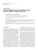
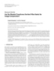
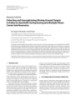
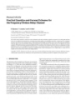
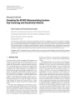
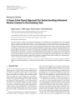
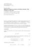
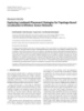
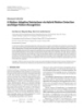
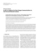
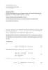
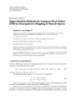
8 EURASIP Journal on Advances in Signal Processing terms, that is, comparing e and 2−B/(N t −1) , we can ﬁnd 2 14 the dominant one. In addition, with this result, we can 12 approximate the achievable rate of the ZF-limited feedback system, which will be provided later in this section. B = 15 10 Based on the distribution of the interference terms, the Rate (bps/Hz) 8 approximation for the achievable rate for the MU mode is given in the following theorem. B = 10 6 Theorem 4. The ergodic achievable rate for the uth user in the 4 MU mode with both delay and channel quantization can be approximated as 2 M −1 2 11 ( j) R(QD) ≈ log2 (e) ai i! · I3 , ,i + 1 , (33) 0 ZF,u α δj 0 5 10 15 20 25 30 35 40 i=0 j =1 SNR, γ (dB) where α = P/U , δ1 = ρu δ , δ2 = e,u , M = Nt − 1, a(1) 2 2 i Simulation and a(2) are given in (E.3), and I3 (·, ·, ·) is given in (A.5) in Approximation i Appendix A. Figure 1: Approximated and simulated ergodic rates for the ZF precoding system with limited feedback, Nt = U = 4. Proof. See Appendix E. The ergodic sum throughput is see that the approximation for the BF system almost matches U the simulation exactly. The approximation for the ZF system R(QD) R(QD) . = (34) is accurate at low to medium SNRs, and becomes a lower ZF,u ZF u=1 bound at high SNR, which is approximately 0.7 bps/Hz in total, or 0.175 bps/Hz per user, lower than the simulation. As a special case, for a ZF system with delay only, we can The throughput of the ZF system is limited by the residual get the following approximation for the ergodic achievable inter-user interference at high SNR, where it is lower than rate. the BF system. This motivates to switch between the SU and Corollary 2. The ergodic achievable rate for the uth user in the MU-MIMO modes. The approximations (19) and (33) will ZF system with delay is approximated as be used to calculate the mode switching points. There may be two switching points for the system with imperfect CSIT, 11 as the SU mode will be selected at both low and high SNR. R(D)u ≈ log2 (e) 2(M −1) · I3 , 2 ,M − 1 , (35) e,u ZF, These two points can be calculated by providing diﬀerent α e,u initial values to the nonlinear equation solver, such as fsolve where α = P/U , M = Nt − 1, and I3 (·, ·, ·) is given in (A.5) in in MATLAB. Appendix A. Proof. Following the same steps in Appendix E with δ1 = 0. 5. Numerical Results In this section, numerical results are presented. First, the operating regions for diﬀerent modes are plotted, which Remark 4. As shown in Lemma 1, the eﬀects of delay and show the impact of diﬀerent parameters, including the channel quantization are equivalent, and so the approxima- normalized Doppler frequency, the codebook size, and the tion in (35) also applies for the limited feedback system. This number of transmit antennas. Then the extension of our is veriﬁed by simulation in Figure 1, which shows that this results for ZF precoding to MMSE precoding is demon- approximation is very accurate and can be used to analyze strated. the limited feedback system. 4.3. Mode Switching. We ﬁrst verify the approximation 5.1. Operating Regions. As shown in Section 4.3, ﬁnding (33) in Figure 2, which compares the approximation with mode switching points requires solving a nonlinear equation, simulation results and the lower bound (29), with B = which does not have a closed-form solution and gives little 10 bits, v = 20 km/hr, fc = 2 GHz, and Ts = 1 msec. We see insight. However, it is easy to evaluate numerically for diﬀerent parameters, from which insights can be drawn. In that the lower bound is very loose, while the approximation is accurate especially for Nt = 2. In fact, the approximation this section, with the calculated mode switching points for diﬀerent parameters, we plot the operating regions for both turns out to be a lower bound. Note that due to the imperfect CSIT, the sum rate reduces with Nt . SU and MU modes. The active mode for the given parameter In Figure 3, we compare the BF and ZF systems, with and the condition to activate each mode can be found from B = 18 bits, fc = 2 GHz, v = 10 km/hr, and Ts = 1 msec. We such plots.
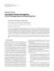
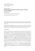
EURASIP Journal on Advances in Signal Processing 9 11 In Figure 4, the operating regions for both SU and MU modes are plotted, for diﬀerent normalized Doppler 10 Nt = U = 2 frequencies and diﬀerent number of feedback bits in Figures 9 4(a) and 4(b), respectively, and with U = Nt = 4. There are analogies between the two plots. Some key observations are 8 Rate (bps/Hz) as follows. 7 Nt = U = 4 (i) For the delay plot in Figure 4(a), comparing the two 6 curves for B = 16 bits and B = 20 bits, we see that the 5 smaller the codebook size, the smaller the operating 4 region for the ZF mode. For the ZF mode to be active, fd Ts needs to be small, speciﬁcally we need 3 Nt = U = 6 fd Ts < 0.055 and fd Ts < 0.046 for B = 20 bits and 2 B = 16 bits, respectively. These conditions are not 1 easily satisﬁed in practical systems. For example, with 0 10 20 30 40 50 60 carrier frequency fc = 2 GHz, mobility v = 20 km/hr, SNR (dB) the Doppler frequency is 37 Hz, and then to satisfy fd Ts < 0.055 the delay should be less than 1.5 msec. ZF (simulation) ZF (approximation) (ii) For the codebook size plot in Figure 4(b), comparing ZF (lower bound) the two curves with v = 10 km/hr and v = 20 km/hr, Figure 2: Comparison of approximation in (33), the lower bound as fd Ts increases (v increases), the ZF operating in (29), and the simulation results for the ZF system with both delay region shrinks. For the ZF mode to be active, we and channel quantization. B = 10 bits, fc = 2 GHz, v = 20 km/hr, should have B ≥ 12 bits and B ≥ 14 bits for and Ts = 1 msec. v = 10 km/hr and v = 20 km/hr, respectively, which means a large codebook size. Note that for BF we only need a small codebook size to get the near-optimal 18 performance [5]. 16 (iii) For a given fd Ts and B, the SU mode will be active at BF region ZF region both low and high SNRs, which is due to its array gain 14 and the robustness to imperfect CSIT, respectively. 12 BF region Rate (bps/Hz) The operating regions for diﬀerent Nt values are shown in 10 Figure 5. We see that as Nt increases, the operating region for the MU mode shrinks. Speciﬁcally, we need B > 12 bits for 8 Nt = 4, B > 19 bits for Nt = 6, and B > 26 bits for Nt = 8 to 6 get the MU mode activated. Note that the minimum required feedback bits per user for the MU mode grow approximately 4 linearly with Nt . 2 0 5.2. ZF versus MMSE Precoding. It is shown in [39] that 0 5 10 15 20 25 30 35 40 45 the regularized ZF precoding, denoted as MMSE precoding SNR (dB) in this paper, can signiﬁcantly increase the throughput at low SNR. In this section, we show that our results on mode BF (simulation) ZF (simulation) BF (approximation) ZF (approximation) switching with ZF precoding can also be applied to MMSE precoding. Figure 3: Mode switching between BF and ZF modes with both CSI ∗ Denote H[n] = [h1 [n], h2 [n], . . . , hU [n]] . Then the delay and channel quantization, B = 18 bits, Nt = 4, fc = 2 GHz, Ts = 1 msec, v = 10 km/hr. MMSE precoding vectors are chosen to be the normalized columns of the matrix [39] −1 U H∗ [n] H[n]H∗ [n] + the eﬀects of delay and quantization are equivalent, so . I (36) P the conclusion will be the same. We see that the MMSE From this, we see that the MMSE precoders converge to ZF precoding outperforms ZF at low to medium SNRs, and precoders at high SNR. Therefore, our derivations for the ZF converges to ZF at high SNR while converges to BF at low system also apply to the MMSE system at high SNR. SNR. In addition, it has the same rate ceiling as the ZF In Figure 6, we compare the performance of ZF and system, and crosses the BF curve roughly at the same point, MMSE precoding systems with delay. Such a comparison can after which we need to switch to the SU mode. Based on also be done in the system with both delay and quantization, this, we can use the second predicted mode switching point which is more time-consuming. As shown in Lemma 1, (the one at higher SNR) of the ZF system for the MMSE
10 EURASIP Journal on Advances in Signal Processing Table 2: Mode switching points. fd Ts = 0.03 fd Ts = 0.04 fd Ts = 0.05 44.2 dB 35.7 dB 29.5 dB MMSE (simulation) 44.2 dB 35.4 dB 28.6 dB ZF (simulation) 41.6 dB 32.9 dB 26.1 dB ZF (calculation) 50 50 45 45 v = 10 km/hr 40 40 ZF region BF region v = 20 km/hr B = 20 35 35 BF region ZF region SNR (dB) SNR (dB) 30 30 ZF region BF region BF region ZF region B = 16 25 25 20 20 15 15 10 10 5 5 10−2 10−1 10 15 20 25 30 Normalised Doppler frequency, fd Ts Codebook size, B (a) Diﬀerent fd Ts (b) Diﬀerent B , fc = 2 GHz, Ts = 1 msec. Figure 4: Operating regions for BF and ZF with both CSI delay and quantization, Nt = 4. 50 18 45 16 40 14 35 12 Nt = U = 4 BF region ZF region Rate (bps/Hz) SNR (dB) Nt = U = 6 30 10 BF region ZF region Nt = U = 8 8 25 6 20 BF region ZF region 4 15 2 10 0 5 −20 −10 0 10 20 30 40 10 15 20 25 30 SNR, γ (dB) Codebook size, B Figure 5: Operating regions for BF and ZF with diﬀerent Nt , fc = MMSE 2 GHz, v = 10 km/hr, Ts = 1 msec. ZF BF Figure 6: Simulation results for BF, ZF and MMSE systems with delay, Nt = U = 4, fd Ts = 0.04. system. We compare the simulation results and calculation results by (21) and (35) for the mode switching points in Table 2. For the ZF system, it is the second switching point; for the MMSE system, it is the only switching point. We 6. Conclusions see that the switching points for MMSE and ZF systems are very close, and the calculated ones are roughly 2.5 ∼ 3 dB In this paper, we compare the SU and MU-MIMO transmis- lower. sions in the broadcast channel with delayed and quantized
EURASIP Journal on Advances in Signal Processing 11 Lemma 2. For a random variable X with probability distribu- CSIT, where the amount of delay and the number of tion function (pdf) fX (x) and cumulative distribution function feedback bits per user are ﬁxed. The throughput of MU- (cdf) FX (x), one has MIMO saturates at high SNR due to residual inter-user interference, for which an SU/MU mode switching algorithm is proposed. We derive accurate closed-form approximations ∞ 1 − FX (x) for the ergodic rates for both SU and MU modes, which are EX [ln(1 + X )] = dx. (A.1) 1+x then used to calculate the mode switching points. It is shown 0 that the MU mode is only possible to be active in the medium SNR regime, with a small normalized Doppler frequency and Proof. The proof follows the integration by parts, a large codebook size. In this paper, we assume that the transmitter knows perfectly the actual received SINR at each active user. In ∞ EX [ln(1 + X )] = ln(1 + x) fX (x)dx practice, there will inevitably be errors in such information 0 due to estimation error and feedback delay, which will result ∞ =− ln(1 + x)[1 − FX (x)] dx in rate mismatch, that is, the transmission rate based on (A.2) 0 the estimated SINR does not match the actual SINR on the ∞ 1 − FX (x) (a) channel, so there will be outage events. How to deal with such = dx, 1+x rate mismatch is of practical importance and we mention 0 several possible approaches as follows. The full investigation of this issue is left to future work. Considering the outage where g is the derivative of the function g , and step (a) events, the transmission strategy can be designed based on follows the integration by parts. the actual information symbols successfully delivered to the receiver, denoted as goodput in [42, 43]. With the estimated SINR, another approach is to back oﬀ on the transmission rate based on the variance of the estimation error, as did in [44, 45] for the single-antenna opportunistic scheduling The following lemma provides some useful integrals for system and in [46] for the multiple-antenna opportunistic rate analysis, which can be derived using the results in [30]. beamforming system. Combined with user selection, the transmission rate can also be determined based on some Lemma 3. lower bound of the actual SINR to make sure that no outage occurs, as did in [47] for the limited feedback system. ∞ xm e−ax For other future work, the MU-MIMO mode studied I1 (a, b, m) = dx in this paper is designed with zero-forcing criterion, which x+b 0 is shown to be sensitive to CSI imperfections, so robust m (k − 1)!(−b)m−k a−k (A.3) precoding design is needed and the impact of the imperfect = CSIT on nonlinear precoding should be investigated. As k=1 power control is an eﬀective way to combat interference, m−1 m ab − (−1) b e E1 (ab), it is interesting to consider the eﬃcient power control algorithm rather than equal power allocation to improve ∞ e−ax I2 (a, b, m) = dx the performance, especially in the heterogeneous scenario. ( x + b )m 0 It is also of practical importance to investigate possible ⎧ approaches to improve the quality of the available CSIT ⎪eab E1 (ab) m = 1, ⎪ ⎪ ⎪ ⎪ with a ﬁxed codebook size, for example, through channel ⎪m−1 ⎪ (A.4) ⎪ (k − 1)! (−a)m−k−1 ⎨ prediction. In this paper, the mode switching algorithm = k=1 (m − 1)! only switches between the SU mode and the MU mode bk ⎪ ⎪ ⎪ ⎪ with Nt users, and how to extend it to allow more MU ⎪ m−1 ⎪ ⎪ + (−a) ⎪ ⎩ m ≥ 2, eab E1 (ab) modes to further improve the performance is currently under (m − 1)! investigation. For practical applications, the impact of more ∞ realistic channel models should also be investigated, such as e−ax I3 (a, b, m) = dx channel correlation. (x + b)m (x + 1) 0 m Appendices (−1)i−1 (1 − b)−i · I2 (a, b, m − i + 1) (A.5) = i=1 A. Useful Results for Rate Analysis + (b − 1)−m · I2 (a, 1, 1), In this appendix, we present some useful results that are used for rate analysis in this paper. where E1 (x) is the exponential-integral function of the ﬁrst The following lemma will be used frequently in the order. derivation of the achievable rate.
12 EURASIP Journal on Advances in Signal Processing B. Proof of Theorem 1 D. Proof of Lemma 1 Let x = hu [n − D] 2 sin2 θ ∼ Γ(M − 1, δ ), y ∼ β(1, M − 2), The average SNR is and x is independent of y . Then the interference term due to 2 (QD) = E P h∗ [n]f (QD) [n] SNRBF quantization is Z = XY . The cdf of Z is 2 ∗ = PE ρh[n − 1] + e[n] h[n − 1] PZ (z) = P x y ≤ z 2 (a) ∗ = PE ρh [n − 1]h[n − 1] ∞ z = FY |X fX (x)dx x 0 2 e∗ [n]h[n − 1] + PE ∞ M −2 z z = 1− 1− fX (x)dx + fX (x)dx x Nt − 1 −B/(Nt −1) (b) z 0 2 ≤ PNt ρ 1 − 2 Nt ∞ ∞ M −2 e−x/δ z xM −2 = fX (x)dx − 1− dx (M − 2)!δ M −1 h∗ [n − 1] · [e[n]e∗ [n]] · h[n − 1] x + PE z 0 ∞ e−(x−z)/δ Nt − 1 −B/(Nt −1) (x − z)M −2 = 1 − e−z/δ (c) dx = PNt ρ2 1 − 2 + P e. 2 (M − 2)!δ M −1 Nt z (B.1) (a) −z/δ = 1−e , As e[n] is independent of h[n − 1], it is also independent of (D.1) h[n − 1], which gives (a). Step (b) follows (12). Step (c) is 2 from the fact e[n] ∼ CN (0, and |h[n − 1]| = 1. 2 e INt ) ∞ M −αy = M !α−(M +1) . ye where step (a) follows the equality 0 C. Proof of Theorem 2 2 E. Proof of Theorem 4 Denote y1 = h[n − 1] 2 and y2 = (1/ e )|e∗ [n]h[n − 1]| , 2 2 2 then y1 ∼ χ2Nt , y2 ∼ χ2 , and they are independent. The Assuming that each interference term in (30) is indepen- received SNR can be written as x = η1 y1 + η2 y2 , where dent of each other and independent of the signal power η1 = Pρ2 and η2 = P e . The cdf of X is given as [48] 2 2 (QD) 2∗ u = u ρu |hu [n − 1]fu [n]| = ρu δ y1 and 2 term, denote Nt / η2 2 e−x/η2 (QD) FX (x) = 1 − ∗ u = u |eu [n]fu [n]| = e,u y2 , then from Lemma 1 we 2 η2 − η1 / 2 2 have y1 ∼ χ2(Nt −1) , and y2 ∼ χ2(Nt −1) as eu [n] is η1 2 and independent of the complex Gaussian with variance e,u + e−x/η1 (C.1) η2 − η1 normalized vector fuQD) [n]. In addition, the signal power ( 2 Nt −1−i i−l Nt −1 i (QD) |h∗ [n]fu [n]| ∼ χ2 . Then the received SINR for the uth 2 η2 x 1 u · . user is approximated as (i − l)! η2 − η1 η1 i=0 l=0 Denote a0 = η2 / (η2 − η1 ) and following Lemma 2 we have αz EX [ln(1 + X )] (QD γZF,u) ≈ x, (E.1) 1 + β δ 1 y 1 + δ2 y 2 ∞ 1 − FX (x) = dx 1+x 0 i−l N −1 i aNt −1−i 1 ∞ 2 2 where α = β = P/U , δ1 = ρu δ , δ2 = e,u , y1 ∼ χ2M , y1 ∼ χ2M , ex/η2 2 2 t N 0 = a0 t dx − (1 − a0 ) 2 M = Nt − 1, z ∼ χ2 , and y1 , y2 , z are independent of each (i − l)! η1 1+x 0 i=0 l=0 other. ∞ xi−l e−x/η1 Let y = δ1 y1 + δ2 y2 , then the pdf of y , which is the sum × dx 1+x of two independent chi-square random variables, is given as 0 [48] 1 N = a0 t I2 , 1, 1 − (1 − a0 ) η2 i−l Nt −1 i aNt −1−i 1 M −1 M −1 1 0 × , 1, i − l , a(1) y i + e− y/δ2 a(2) y i pY y = e− y/δ1 I1 (i − l)! η1 η1 i i i=0 l=0 i=0 i=0 (C.2) (E.2) 2 M −1 where I1 (·, ·, ·) and I2 (·, ·, ·) are given in (A.3) and (A.4), − y/δ j ( j ) i = e ai y , respectively. j =1 i=0
EURASIP Journal on Advances in Signal Processing 13 References where M δ1 1 [1] E. Telatar, “Capacity of multi-antenna Gaussian channels,” a(1) = i δ1+1 (M − 1)! δ1 − δ2 i European Transactions on Telecommunications, vol. 10, no. 6, pp. 585–595, 1999. M −1−i (2(M − 1) − i)! δ2 [2] A. Goldsmith, S. A. Jafar, N. Jindal, and S. Vishwanath, × , i!(M − 1 − i)! δ2 − δ1 “Capacity limits of MIMO channels,” IEEE Journal on Selected (E.3) Areas in Communications, vol. 21, no. 5, pp. 684–702, 2003. M δ2 1 a(2) [3] D. Gesbert, M. Kountouris, R. W. Heath Jr., C. B. Chae, and = i+1 i δ2 (M − 1)! δ2 − δ1 T. Salzer, “Shifting the MIMO paradigm: from single user to multiuser communications,” IEEE Signal Processing Magazine, M −1−i (2(M − 1) − i)! δ1 vol. 24, no. 5, pp. 36–46, 2007. × . i!(M − 1 − i)! δ1 − δ2 [4] B. Hassibi and M. Sharif, “Fundamental limits in MIMO broadcast channels,” IEEE Journal on Selected Areas in Com- The cdf of X is munications, vol. 25, no. 7, pp. 1333–1344, 2007. αz [5] D. J. Love, R. W. Heath Jr., W. Santipach, and M. L. Honig, FX (x) = P ≤x “What is the value of limited feedback for MIMO channels?” 1 + βy IEEE Communications Magazine, vol. 42, no. 10, pp. 54–59, ∞ x 2004. = FZ |Y 1 + βy pY y d y α [6] D. J. Love, R. W. Heath Jr., V. K. N. Lau, D. Gesbert, B. D. Rao, 0 and M. Andrews, “An overview of limited feedback in wireless ∞ 1 − e−(x/α)(1+βy) pY y d y = communication systems,” IEEE Journal on Selected Areas in Communications, vol. 26, no. 8, pp. 1341–1365, 2008. 0 ∞ [7] N. Jindal, “MIMO broadcast channels with ﬁnite-rate feed- = 1 − e−x/α e−βxy/α pY y d y back,” IEEE Transactions on Information Theory, vol. 52, no. 0 11, pp. 5045–5060, 2006. ⎧ ⎫ ∞⎨ 2 M −1 ⎬ [8] P. Ding, D. J. Love, and M. D. Zoltowski, “Multiple antenna β 1 ( j) −x/α y ai y i ⎭d y = 1− e exp − x + broadcast channels with shape feedback and limited feedback,” 0 ⎩ j =1 i=0 α δj IEEE Transactions on Signal Processing, vol. 55, no. 7, pp. 3417– ⎡ ⎤ 3428, 2007. 2 M −1 ( j) ⎢ ⎥ ai i! [9] R. W. Heath Jr. and A. J. Paulraj, “Switching between diversity (a) = 1 − e−x/α ⎣ i+1 ⎦, and multiplexing in MIMO systems,” IEEE Transactions on β/α x + 1/δ j j =1 i=0 Communications, vol. 53, no. 6, pp. 962–972, 2005. (E.4) [10] D. J. Love and R. W. Heath Jr., “Multi-mode precoding using linear receivers for limited feedback MIMO systems,” in Pro- ∞ where step (a) follows the equality 0 y M e−αy = M !α−(M +1) . ceedings of IEEE International Conference on Communications Then the ergodic achievable rate for the uth user is (ICC ’04), vol. 1, pp. 448–452, Paris, France, June 2004. approximated as [11] R. W. Heath Jr. and D. J. Love, “Multimode antenna selection for spatial multiplexing systems with linear receivers,” IEEE R(QD) = Eγ log2 1 + γZF,u) (QD ZF,u Transactions on Signal Processing, vol. 53, no. 8, pp. 3042–3056, 2005. ≈ log2 (e)EX [ln(1 + X )] [12] J. C. Roh and B. D. Rao, “Design and analysis of MIMO ∞ spatial multiplexing systems with quantized feedback,” IEEE 1 − FX (x) (a) = log2 (e) dx Transactions on Signal Processing, vol. 54, no. 8, pp. 2874–2886, x+1 0 2006. ⎡ ⎤ [13] N. Ravindran and N. Jindal, “Limited feedback-based block ∞ M −1 2 e−x/α ⎢ ( j) α ⎥ = log2 (e) ⎣ai i! ⎦dx diagonalization for the MIMO broadcast channel,” IEEE i+1 β 0 i=0 j =1 Journal on Selected Areas in Communications, vol. 26, no. 8, pp. x + α/βδ j (x +1) 1473–1482, 2008. ⎡ ⎤ i+1 M −1 2 [14] T. Yoo, N. Jindal, and A. Goldsmith, “Multi-antenna downlink ⎣a( j ) i! α 1α , i + 1 ⎦, (b) = log2 (e) I3 , channels with limited feedback and user selection,” IEEE i β α βδ j i=0 j =1 Journal on Selected Areas in Communications, vol. 25, no. 7, pp. (E.5) 1478–1491, 2007. [15] G. Caire, “MIMO downlink joint processing and scheduling: where step (a) follows from Lemma 2, step (b) follows the a survey of classical and recent results,” in Proceedings of the expression of I3 (·, ·, ·) in (A.5). For equal power allocation, Workshop on Information Theory and Its Applications (ITA ’06), α = β = P/U , and the expression can be simpliﬁed into (33). San Diego, Calif, USA, January 2006. [16] G. Caire, N. Jindal, M. Kobayashi, and N. Ravindran, “Mul- Acknowledgment tiuser MIMO achievable rates with downlink training and channel state feedback,” submitted to IEEE Transactions on This work has been supported in part by AT&T Labs, Inc. Information Theory, November 2007.
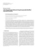
14 EURASIP Journal on Advances in Signal Processing [17] G. Caire, N. Jindal, and S. Shamai, “On the required accuracy [32] M. H. M. Costa, “Writing on dirty paper,” IEEE Transactions of transmitter channel state information in multiple antenna on Information Theory, vol. 29, no. 3, pp. 439–441, 1983. broadcast channels,” in Proceedings of IEEE Asilomar Confer- [33] G. Caire and S. Shamai (Shitz), “On the achievable throughput ence on Signals, Systems and Computers, pp. 287–291, Paciﬁc of a multiantenna Gaussian broadcast channel,” IEEE Trans- Grove, Calif, USA, November 2007. actions on Information Theory, vol. 49, no. 7, pp. 1691–1706, [18] R. de Francisco and D. T. M. Slock, “A design framework 2003. for scalar feedback in MIMO broadcast channels,” EURASIP [34] W. Yu and J. Cioﬃ, “The sum capacity of a Gaussian vector Journal on Advances in Signal Processing, vol. 8, no. 1, pp. 1– broadcast channel,” IEEE Transactions on Information Theory, 12, 2008. vol. 50, no. 9, pp. 1875–1892, 2004. [19] E. A. Jorswieck, P. Svedman, and B. Ottersten, “Performance of [35] S. Vishwanath, N. Jindal, and A. Goldsmith, “Duality, TDMA and SDMA based opportunistic beamforming,” IEEE achievable rates, and sum-rate capacity of Gaussian MIMO Transactions on Wireless Communications, vol. 7, no. 11, pp. broadcast channels,” IEEE Transactions on Information Theory, 4058–4063, 2008. vol. 49, no. 10, pp. 2658–2668, 2003. [20] M. Kountouris, D. Gesbert, and T. S¨ lzer, “Distributed trans- a [36] P. Viswanath and D. N. C. Tse, “Sum capacity of the vector mit mode selection for MISO broadcast channels with limited Gaussian broadcast channel and uplink-downlink duality,” feedback: switching from SDMA to TDMA,” in Proceedings IEEE Transactions on Information Theory, vol. 49, no. 8, pp. of IEEE Workshop on Signal Processing Advances in Wireless 1912–1921, 2003. Communications (SPAWC ’08), pp. 371–375, Recife, Brazil, [37] H. Weingarten, Y. Steinberg, and S. Shamai, “The capacity July 2008. region of the Gaussian multiple-input multiple-output broad- [21] N. Ravindran, N. Jindal, and H. C. Huang, “Beamforming cast channel,” IEEE Transactions on Information Theory, vol. with ﬁnite rate feedback for LOS MIMO downlink channels,” 52, no. 9, pp. 3936–3964, 2006. in Proceedings of IEEE Global Telecommunications Conference [38] N. Jindal, “A high SNR analysis of MIMO broadcast channels,” (GLOBECOM ’07), pp. 4200–4204, Washington, DC, USA, in Proceedings of IEEE International Symposium on Information November 2007. Theory (ISIT ’05), pp. 2310–2314, Adelaide, Australia, Septem- [22] S. Haykin, Adaptive Filter Theory, Prentice-Hall, Englewood ber 2005. Cliﬀs, NJ, USA, 3rd edition, 1996. [39] C. B. Peel, B. M. Hochwald, and A. L. Swindlehurst, “A [23] R. H. Clarke, “A statistical theory of mobile radio reception,” vector-perturbation technique for near-capacity multiantenna Bell System Technical Journal, vol. 47, pp. 957–1000, 1968. multiuser communication—part I: channel inversion and [24] E. N. Onggosanusi, A. Gatherer, A. G. Dabak, and S. Hosur, regularization,” IEEE Transactions on Communications, vol. 53, “Performance analysis of closed-loop transmit diversity in the no. 1, pp. 195–202, 2005. presence of feedback delay,” IEEE Transactions on Communi- [40] K. K. Mukkavilli, A. Sabharwal, E. Erkip, and B. Aazhang, “On cations, vol. 49, no. 9, pp. 1618–1630, 2001. beamforming with ﬁnite rate feedback in multiple-antenna [25] H. T. Nguyen, J. B. Andersen, and G. F. Pedersen, “Capacity systems,” IEEE Transactions on Information Theory, vol. 49, no. and performance of MIMO systems under the impact of feed- 10, pp. 2562–2579, 2003. back delay,” in Proceedings of IEEE International Symposium on [41] S. Zhou, Z. Wang, and G. B. Giannakis, “Quantifying the Personal, Indoor and Mobile Radio Communications (PIMRC power loss when transmit beamforming relies on ﬁnite-rate ’04), vol. 1, pp. 53–57, Barcelona, Spain, September 2004. feedback,” IEEE Transactions on Wireless Communications, vol. [26] G. Caire, N. Jindal, M. Kobayashi, and N. Ravindran, “Quan- 4, no. 4, pp. 1948–1957, 2005. tized vs. analog feedback for the MIMO broadcast channel: a [42] V. K. N. Lau and M. Jiang, “Performance analysis of multiuser comparison between zero-forcing based achievable rates,” in downlink space-time scheduling for TDD systems with imper- Proceedings of IEEE International Symposium on Information fect CSIT,” IEEE Transactions on Vehicular Technology, vol. 55, Theory (ISIT ’07), pp. 2046–2050, Nice, France, June 2007. no. 1, pp. 296–305, 2006. [27] M. Kobayashi and G. Caire, “Joint beamforming and schedul- ing for a multi-antenna downlink with imperfect transmitter [43] T. Wu and V. K. N. Lau, “Robust rate, power and precoder channel knowledge,” IEEE Journal on Selected Areas in Com- adaptation for slow fading MIMO channels with noisy limited munications, vol. 25, no. 7, pp. 1468–1477, 2007. feedback,” IEEE Transactions on Wireless Communications, vol. 7, no. 6, pp. 2360–2367, 2008. [28] W. Santipach and M. L. Honig, “Asymptotic capacity of [44] A. Vakili, M. Sharif, and B. Hassibi, “The eﬀect of channel beamforming with limited feedback,” in Proceedings of IEEE International Symposium on Information Theory (ISIT ’04), p. estimation error on the throughput of broadcast channels,” 290, Chicago, Ill, USA, June-July 2004. in Proceedings of IEEE International Conference on Acoustics, Speech, and Signal Processing (ICASSP ’06), vol. 4, pp. 29–32, [29] C. K. Au-Yeung and D. J. Love, “On the performance of ran- Toulouse, France, May 2006. dom vector quantization limited feedback beamforming in a MISO system,” IEEE Transactions on Wireless Communications, [45] A. Vakili and B. Hassibi, “On the throughput of broadcast vol. 6, no. 2, pp. 458–462, 2007. channels with imperfect CSI,” in Proceedings of IEEE Workshop on Signal Processing Advances in Wireless Communications [30] I. S. Gradshteyn and I. M. Ryzhik, Table of Integrals, Series, and (SPAWC ’06), pp. 1–5, Cannes, France, July 2006. Products, Academic Press, San Diego, Calif, USA, 5th edition, 1994. [46] A. Vakili, A. F. Dana, and B. Hassibi, “On the throughput [31] M.-S. Alouini and A. J. Goldsmith, “Capacity of Rayleigh of opportunistic beamforming with imperfect CSI,” in Pro- fading channels under diﬀerent adaptive transmission and ceedings of the ACM International Wireless Communications diversity-combining techniques,” IEEE Transactions on Vehic- and Mobile Computing Conference (IWCMC ’07), pp. 19–23, ular Technology, vol. 48, no. 4, pp. 1165–1181, 1999. Honolulu, Hawaii, USA, August 2007.
EURASIP Journal on Advances in Signal Processing 15 [47] M. Kountouris, R. de Francisco, D. Gesbert, D. T. M. Slock, and T. Salzer, “Eﬃcient metrics for scheduling in MIMO broadcast channels with limited feedback,” in Proceedings of IEEE International Conference on Acoustics, Speech, and Signal Processing (ICASSP ’07), vol. 3, pp. 109–112, Honolulu, Hawaii, USA, April 2007. [48] M. K. Simon, Probability Distributions Involving Gaussian Random Variables: A Handbook for Engineers and Scientists, Springer, New York, NY, USA, 2002.