Báo cáo hóa học: " Research Article Real-Time Guitar Preamp Simulation Using Modiﬁed Blockwise Method and Approximations Jaromir Macak and Jiri Schimmel"

Chia sẻ: Nguyen Minh Thang | Ngày: | Loại File: PDF | Số trang:11

Thêm vào BST

Báo xấu

37
lượt xem 6
download

Download Vui lòng tải xuống để xem tài liệu đầy đủ

Tuyển tập báo cáo các nghiên cứu khoa học quốc tế ngành hóa học dành cho các bạn yêu hóa học tham khảo đề tài: Research Article Real-Time Guitar Preamp Simulation Using Modiﬁed Blockwise Method and Approximations Jaromir Macak and Jiri Schimmel

Chủ đề:

Bình luận(0) Đăng nhập để gửi bình luận!

Lưu

Nội dung Text: Báo cáo hóa học: " Research Article Real-Time Guitar Preamp Simulation Using Modiﬁed Blockwise Method and Approximations Jaromir Macak and Jiri Schimmel"

Hindawi Publishing Corporation EURASIP Journal on Advances in Signal Processing Volume 2011, Article ID 629309, 11 pages doi:10.1155/2011/629309 Research Article Real-Time Guitar Preamp Simulation Using Modiﬁed Blockwise Method and Approximations Jaromir Macak and Jiri Schimmel Faculty of Electrical Engineering and Communication, Brno University of Technology, 61600 Brno, Czech Republic Correspondence should be addressed to Jaromir Macak, jaromir.macak@phd.feec.vutbr.cz Received 14 September 2010; Revised 12 December 2010; Accepted 27 January 2011 Academic Editor: Vesa Valimaki Copyright © 2011 J. Macak and J. Schimmel. This is an open access article distributed under the Creative Commons Attribution License, which permits unrestricted use, distribution, and reproduction in any medium, provided the original work is properly cited. The designing of algorithms for real-time digital simulation of analog eﬀects and ampliﬁers brings two contradictory requirements: accuracy versus computational eﬃciency. In this paper, the simulation of a typical guitar tube preamp using an approximation of the solution of diﬀerential equations is discussed with regard to accuracy and computational complexity. The solution of circuit equations is precomputed and stored in N-D tables. The stored values are approximated, and therefore diﬀerent approximation techniques are investigated as well. The approximated functions are used for output signal computation and also for circuit state update. The designed algorithm is compared to the numerical solution of the given preamp and also to the real preamp. 1. Introduction with a grid current is presented in [7]. A decomposition into a linear dynamic and a nonlinear static part is used in The real-time digital simulation of analog guitar eﬀects and nonlinear state-space formulations [8, 9] and this method ampliﬁers has always been, unfortunately, a compromise was automated in [10], where the algorithm parameters between accuracy and speed of a simulation algorithm. are derived from the SPICE netlist. An extended state- There are many diﬀerent approaches to the simulation, space representation was used in [11] for guitar poweramp such as a black box approach, a white box (informed) simulation. A direct solution of nonlinear circuit ordinary diﬀerential equations (ODEs) was used in [2, 12], but approach, circuit-based approaches, and so forth [1]. All these algorithms diﬀer in accuracy of the simulation as well as the computational requirements are high. Therefore, an approximation of the solution of ODEs was used in [13]. in computational complexity. The circuit-based techniques usually oﬀer the best accuracy because a simulated circuit However, an approximation of nonlinear functions are also is exactly described by circuit equations, which are often used in [6, 10]. diﬀerential equations. Nevertheless, the computational com- In this paper, a typical guitar preamp is simulated using the approximation of a solution of diﬀerential equations. plexity needed for a solution of these equations is very high [2]. Hence, more eﬃcient algorithms for the solution of First of all, the guitar preamp is decomposed into separate the equations must be found. This can often be made by blocks. It is necessary to ﬁnd a proper division, because it can inﬂuence the accuracy of the whole simulation. A commonly neglecting unimportant factors, for example, tube heating, decomposing into separate blocks [3], and decomposing used division into blocks does not consider mutual interac- into a linear and nonlinear part. Subsequently, the separate tions between connected blocks. As was shown in [13, 14], the simulation fails especially if the load of the simulated simpliﬁed block can be described by a new set of circuit block is nonlinear, which is typical for circuits with tubes. equations that can be solved using several methods, for example, digital ﬁlters and waveshaping [3], Hammerstein Therefore, a modiﬁcation designed in [13] and investigated model [4]. The triode ampliﬁer simulation using wave digital in [14] must be used in order to get good simulation results if the blocks are highly nonlinear and connected in series. After ﬁlters is described in [5, 6] and an enhanced tube model
2 EURASIP Journal on Advances in Signal Processing the decomposition, the new set of diﬀerential equations is Table 1: Values for circuit elements for Figure 1. approximated according to [13]. The chosen approximation R1 Rg 1 Rk 1 R p1 R2 Rg 2 markedly aﬀects the accuracy of the algorithm as well as 68 kΩ 1 MΩ 2.7 kΩ 100 kΩ 470 kΩ 1 MΩ the computational complexity. Therefore, several types of Rk2 Rp2 R3 Rg3 Rk3 Rp3 approximations will be discussed. 1.8 kΩ 100 kΩ 470 kΩ 470 kΩ 1.8 kΩ 100 kΩ Considering real-time simulation, the computational R4 Rg4 Rk4 Rp4 RL — complexity must be investigated. Commonly used electronic 470 kΩ 470 kΩ 1.8 kΩ 100 kΩ 4 MΩ — circuit simulators has a computational complexity given by O(N 1.4 ) where N is the number of circuit nodes [1]. C1 C2 C3 C4 Vss — However, this notation does not determine the real compu- 1 µF 22 nF 22 nF 22 nF 400 V — tational complexity, that is, the real number of mathematical operations of the algorithm. Thus in this paper, the whole guitar preamp is numerically simulated using a similar found in [13]. The ﬁnal circuit equations describing the circuit in Figure 1 are approach as in the electronic circuit simulators and the number of instructions required for one signal sample is 0 = Vin − Vg 1 G1 − Vg 1 Gg 1 − ig 1 , computed. It is compared to the number of instructions of the numerical simulation based on the division into blocks Vk Gk − i p1 − ig 1 and also to the number of instructions of the approximated 0 = Vc1m − Vc1 − , C1 fs solution of the given circuit. Finally, the accuracy of the numerical simulation of the 0 = Vss − V p1 G p1 − V2 − Vg 2 G2 − i p1 , whole preamp must be compared to the simulation using approximation and also to a real guitar preamp. V2 − Vg 2 G2 0 = Vc2m − Vc2 − , C2 fs 2. Guitar Preamp Simulation 0 = V2 − Vg 2 G2 − Vg 2 Gg 2 − ig 2 , A guitar tube preamp usually consists of several triode ampliﬁers connected in series. The separate triode ampliﬁers 0 = Vk2 Gk2 − ig 2 − i p2 , are decoupled using decoupling capacitors in order to remove DC. The number of triode ampliﬁers in the circuit 0 = Vss − V p2 G p2 − V3 − Vg 3 G3 − i p2 , depends on a given topology and therefore it can diﬀer for diﬀerent preamps. Guitar preamps usually contain two to ﬁve V3 − Vg 3 G3 (1) triode ampliﬁers. They are usually connected as a common- 0 = Vc3m − Vc3 − , C3 fs cathode ampliﬁer. However, the preamp can also contain a cathode follower (e.g., Marshall). The circuit schematic of 0 = V3 − Vg 3 G3 − Vg 3 Gg 3 − ig 3 , a testable guitar tube preamp is shown in Figure 1 and the values for circuit elements are listed in Table 1. The values 0 = Vk3 Gk3 − ig 3 − i p3 , were chosen as typical values for tube circuits. This preamp consists of four common-cathode triode ampliﬁers. This 0 = Vss − V p3 G p3 − V4 − Vg 4 G4 − i p3 , circuit schematic is similar to circuit schematics that are used in some real “Hi Gain” guitar ampliﬁers (e.g., Mesa Boogie V4 − Vg 4 G4 or Engl). Only the values of the circuit elements can have 0 = Vc4m − Vc4 − , C4 fs diﬀering values, some of the common-cathode ampliﬁers can have a cathode capacitor to gain the high frequencies 0 = V4 − Vg 4 G4 − Vg 4 Gg 4 − ig 4 , and a potentiometer “Gain” with a capacitor connected between terminals of the potentiometer are used instead of 0 = Vk4 Gk4 − ig 4 − i p4 , resistors R2 and Rg 2 (see Figure 1). However, the frequency dependence of the “Gain” parameter caused by the capacitor 0 = Vss − V p4 G p4 − V p4 GL − i p4 , can be simulated by a linear ﬁlter. In order to simulate the preamp from Figure 1, an where ig is the grid current function ig (Ug − Uk ) and ia is the analysis of the circuit must be done. The circuit equations plate current function ia (Ug − Uk , Ua − Uk ). The symbol G can be obtained using nodal analysis. In this case, Kirchhoﬀ¨ ı represents the conductance of the resistors from the circuit Current Law (KCL) is used. After obtaining circuit equations, schematic in Figure 1, fs is the sampling frequency, Vss is the a discretization of diﬀerential equations is realized. The power supply, and Vin is the input voltage. Voltages Vc1m , backward Euler method with step of a sampling period was Vc2m , Vc3m , and Vc4m are the voltages on the capacitors in used. Naturally, a diﬀerent method for discretization can be the previous signal sampling period. Equations (1) have 15 used, however, this method was chosen due to its simplicity. unknown voltage variables (denoted in Figure 1); 1st, 5th, More information about obtaining the equations can be 9th, 13th equations describe grid nodes of all tubes four
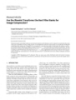
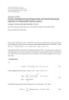
EURASIP Journal on Advances in Signal Processing 3 Vss Gain R p1 R p2 R p3 R p4 potentiometer V p1 V2 V p2 V3 V p3 V4 V p4 R2 R3 R4 Vg 1 C2 C4 C3 Vg 3 Vg 4 Vg 2 Vin R1 Vk2 Vk3 Vk4 Vk1 Rg 1 Rk 1 C1 Rg 2 Rk2 Rg 3 Rk3 Rg 4 Rk 4 RL Figure 1: A guitar tube preamp circuit schematic. tubes; 2nd, 6th, 10th, and 14th equations are cathode nodes of nonlinear device model functions (2) and (4) as c p and cg respectively, the total cost of the function F(xn ) is c f = i and 3rd, 7th, 11th, 15th equations are anode nodes. Koren’s i nonlinear model of a triode has been used in this paper [15]. 78 + 4c p + 4cg operations. The Jacobian matrix J(xn ) contains i The triode plate current is given by partial ﬁrst-order derivation of the function F(xn ). Since i ) has not been a continuous function, the function F(xn E E1 x the derivations are computed for instance using the ﬁnite ia = 1 + sgn(E1 ) , (2) diﬀerence formula Kg 1 1 where f (x) = f (x + h) − f (x) (6) ⎛ ⎛ ⎛ ⎞⎞⎞ h Ugk Uak 1 log⎝1 + exp⎝K p ⎝ + ⎠⎠⎠. E1 = (3) i with a step h that consists of two function calls F(xn ) and Kp µ 2 Kvb + Uak two add operations and one multiply operation. The total cost of the Jacobian matrix computation is N + 1 function Parameters µ, Ex , Kg 1 , Kg 2 , K p , and Kvb , are available in [15], calls resulting in (c f + 3)N operations. When the Jacobian Ugk is the grid-to-cathode voltage and Uak is the plate-to- matrix is established, its inversion matrix is computed. The cathode voltage. The grid current is not speciﬁed in [15], computational complexity depends on the chosen algorithm and therefore the grid model was adopted from the Microcap of the matrix inversion. Generally, it is a O(N 3 ) problem. simulator [16]. The grid current is However, the LU decomposition oﬀers a more eﬃcient ⎧ implementation. Then, (5) is rewritten as ⎪ 3/ 2 ⎨gc f ugk − gco ugk ≥ gco , , ig = ⎪ (4) ⎩ ugk < gco , 0, i LU = J xn , (7) where gc f = 1 · 10−5 and gco = −0.2. Frequency properties i Ly = F xn , (8) of the tube (e.g., Miller capacitance) are not considered in UΔxn = y, the simulation due to simplicity of tube model. However, i (9) it inﬂuences accuracy of the simulation, because the Miller xn+1 = xn − Δxn . i i i capacitance makes a low-pass ﬁlter at the input of the tube. (10) [17] Generally, a system of nonlinear equation (1) is solved According to [18], the cost of (7) (Crout’s algorithm) is using the Newton-Raphson method (1/ 3)N 3 of inner loops containing one multiply and add operation, the cost of (8) and (9) is N 2 multiply and add xn+1 = xn − J−1 xn F xn , i i i i (5) operations. Thus, the total cost is cLU = (2/ 3)N 3 + 4N 2 operations. Knowing Δxn , (10) can be solved, which requires i i i where xn is a vector of unknown voltages, J(xn ) is the N add operations. The total cost of the Newton method is i ) is the function given by (1), i Jacobian matrix, and F(xn then denotes iteration index and n is the time index. 2 However, if it is a real-time simulation, computational c f + 3 N + c f + N 3 + 4N 2 + N , cnm = i (11) demand has to be investigated. According to (1), the function 3 i F(xn ) involves four grid functions (4), four plate functions where i is a number of iterations of the Newton method (2), 47 add operations, and 31 multiply operations if the sampling frequency fs is substituted with the sample period and N is the number of circuit nodes. However, it must be Ts = 1/ fs and values of capacitors are substituted with said that this number is theoretical. Neither of the algorithm the reciprocal values. Considering the computational cost branches nor memory movements have been considered.
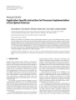
4 EURASIP Journal on Advances in Signal Processing The circuit is described by Triode Triode amp. 1 amp. 2 0 = Vin − Vg 1 G1 − Vg 1 Gg 1 − ig 1 , Triode Triode Vk Gk − i p1 − ig 1 amp. 2 amp. 3 0 = Vc1m − Vc1 − , C1 fs Triode Triode amp. 3 amp. 4 0 = Vss − V p1 G p1 − V2 − Vg 2 G2 − i p1 , Figure 2: Preamp block decomposition using modiﬁed blockwise V2 − Vg 2 G2 (12) method [13]. 0 = Vc2m − Vc2 − , C2 fs 0 = V2 − Vg 2 G2 − Vg 2 Gg 2 − ig 2 , Vss R p1 R p2 0 = Vk2 Gk2 − ig 2 − i p2 , V p1 V2 V p2 0 = Vss − V p2 G p2 − V p2 GL − i p2 . R2 Vg 1 C2 Vg 2 The function F(xn ) involves 15 multiply operations and 22 Vin R1 add operations and four nonlinear function calls resulting Vk2 in c f = 37 + 2c p + 2cg operations. The equation is solved Vk1 using the Newton method as well. Therefore, (11) can be C1 Rg 1 Rk 1 Rg 2 Rk2 RL used for the determination of the computational complexity. For given N = 7, the total cost is cnm = i 749 + 16 cg + c p . (13) Figure 3: Circuit schematic of the ﬁrst block of the guitar preamp. Figure 4 shows the circuit schematic of the second and third block. The circuit elements values can be derived from Table 1. The block contains two common-cathode tube 3. Simulation Using Modiﬁed ampliﬁers without the cathode capacitor. The output signal Blockwise Method is obtained from the node V2 . The computational complexity is similar to the ﬁrst The simulated circuit can also be divided into blocks. An block. They only diﬀer in the function F(xn ), because the example of division into blocks using the modiﬁed blockwise cathode capacitor in the ﬁrst ampliﬁer is missing (circuit method [14] is shown in Figure 2. The whole circuit from equations are not explicitly shown). Therefore, it has c f = Figure 1 is divided into three separate blocks containing two 34 + 2c p + 2cg operations in this case. The cost is then tubes in this case. Two types of blocks are used. The ﬁrst one contains the common-cathode tube ampliﬁer with a cnm = i 728 + 16 cg + c p . (14) cathode capacitor and is used as the ﬁrst block in Figure 2. The other one contains the common-cathode tube ampliﬁer If the blocks are connected together, the total cost of the without the cathode capacitor and is used as the second solution of these blocks is and third block. Then, the simulation requires a solution of three independent simpler blocks, and as a result the cnm = i1 749 + 16 cg + c p + computational complexity can be lower. (15) The circuit schematic of the ﬁrst block is shown in + (i2 + i3 ) 728 + 16 cg + c p , Figure 3. It consists of two common-cathode tube ampliﬁers, the ﬁrst tube ampliﬁer is connected exactly according to the where i1 , i2 , and i3 are numbers of iterations of the ﬁrst, circuit schematic in Figure 1. The second tube ampliﬁer is second, and third block, respectively. similar to the second tube ampliﬁer in 1, only the second decoupling capacitor is not included and the load resistor 4. Simulation Using Modiﬁed Blockwise RL is connected directly to plate of the second tube. This Method and Approximation can be done, because the value of resistor RL and presence of decoupling capacitor have very low inﬂuence on the ﬁrst A system of diﬀerential equations can be described by the preamp [14] because the output signal is obtained at the equation output of the ﬁrst ampliﬁer and the second ampliﬁer builds only the load of the ﬁrst ampliﬁer. The value of resistor RL is 0 = F(Vin , Vc1 , Vc2 , . . . , VcM ), (16) 4 MΩ and the others circuit elements values can be obtained where Vin is an input voltage or an input signal value and from Table 1. The output signal voltage is obtained from the node V2 . Vc1 , Vc2 , . . . , VcM are voltages on capacitors. Thus, the system
EURASIP Journal on Advances in Signal Processing 5 Vss i where Vout are precomputed output values, i is index into a vector of fprecomputed output values and p is R p1 R p2 a fractional part between neighbouring precomputed values [19]. The linear interpolation consists of two V p1 V p2 V2 add operations, two multiply operations, index and R2 Vg 1 C2 fractional part computation. The bilinear interpola- Vg 2 Vin tion has to be used as the approximating function R1 for the ﬁrst-order diﬀerential system, because the Vk2 Vk1 system has two inputs: input signal and the capacitor voltage. The bilinear interpolation requires three lin- Rg 1 Rk1 Rg 2 Rk2 RL ear interpolations (18). Generally, the N -dimensional linear interpolation must be used, if there are M accumulation elements. It requires 2N − 1 linear interpolations. Figure 4: Circuit schematic of the second block of the guitar preamp. (ii) Spline Interpolation oﬀers the smooth behavior of an approximating function. The spline interpolation is given by has N = M +1 inputs and also N outputs—an output voltage or an output signal level and new voltages on the capacitors. 3 1 + p − 4 p3 i p3 i−1 Vout = Vout + Vout The system has a particular solution for a combination of the 6 6 inputs. The solution can be precomputed for certain combi- 3 3 3 2−p −4 1− p 1− p nations of the input voltages and it must be approximated, i+1 i+2 Vout + Vout , + because the solution has to involve all combinations of the 6 6 input voltages [13]. The output signal value is computed on (19) the basis of the approximated solution. Then, the state of the circuit (capacitor voltages) is actualized. The new capacitor where p is the fractional part between neighbouring voltages are used as the inputs for the next sample period. precomputed values [19]. It consists of 10 add oper- The approximation leads to the following set of equations: ations and 19 multiply operations, index and frac- tional part computation. The N -dimensional spline n n Vout = Fout Vin , Vcn , Vcn , . . . , VcM , n interpolation requires (4N −1)/ 3 spline interpolations 1 2 (19). n n Vuc+1 = Vuc1 + Ts Fc1 Vin , Vcn , Vcn , . . . , VcM , n n 1 1 2 (iii) Cubic Spline Approximation also oﬀers the smooth n n Vuc+1 = Vuc2 + Ts Fc2 Vin , Vcn , Vcn , . . . , VcM , n n (17) behavior of approximating function but compared 2 1 2 to the spline interpolation, coeﬃcients of cubic . . polynomials are stored instead of the precomputed . values. The cubic polynomial is given by n+1 n n n VucM = VucM + Ts FcN Vin , Vcn , Vcn , . . . , VcM , 1 2 3 i 2 Vout = a j Vin + b j Vin + c j Vin + d j where functions Fout , Fuc1 , Fuc2 , . . . , FucM are approximating (20) = functions, Ts is the sample period, and the superscript n a j Vin + b j Vin + c j Vin + d j , denotes time index. The function Fout approximates directly where j index is into a vector of polynomial coeﬃ- the output signal value and the functions Fuc1 , Fuc2 , . . . , FucM cients [20]. It consists of three add operations and approximate changes of the capacitor voltage. The compu- three multiply operations. The combination of spline tational complexity depends on the number of accumula- and linear approximation can be used for the higher- tion circuit elements (capacitors) N . The computation of order system simulation, because the functions that one output signal sample requires M , add operations, M , are being approximated have very similar shape multiply operations and N , computations of approximating with diﬀerent capacitor voltages Vc1 , Vc2 , . . . , VcN , functions. Therefore, the total computational complexity as shown in simulations in [13]. The splines are markedly depends on the chosen approximation. Further- used for diﬀerent input signal values and the linear more, the chosen approximation inﬂuences the accuracy of interpolation (18) for diﬀerent capacitor voltages. the algorithm and also memory requirements. Two spline approximations (20) and one linear (i) Linear Interpolation oﬀers the fastest implementa- interpolation (18) are required for the ﬁrst-order system (N = 2). Generally, it requires 2(N −1) − 1 linear tion. However, it requires many precomputed values interpolations and 2(N −1) spline approximations. for smooth behavior. The linear interpolation is given by All approximations and interpolations work with indexes into a vector of spline coeﬃcients or precomputed values of i i+1 Vout = Vout 1 − p + Vout p, (18)
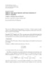
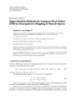
6 EURASIP Journal on Advances in Signal Processing the solution of the system. It is necessary to ﬁnd eﬃcient Table 2: Lookup table for simulation of the ﬁrst block (size 2 MB). determination of the index, if it is real-time simulation. The Variable Min. Max. Step fastest way of determination of the index is computation −200 Vin [V] 200 1 directly from the input values. The solution of the system is VC 1 [V] 0 5 5 precomputed for integer values of the inputs. Then the index VC 2 [V] 0 400 5 is obtained from i = Vin (21) Table 3: Look-up table for simulation of the second and third block (size 1 MB). and the fractional part is obtained from Variable Min. Max. Step p = Vin − i. (22) −200 Vin [V] 200 1 The system of (12) has three inputs (input voltage and VC 1 [V] 0 400 5 two input voltages on capacitors), and therefore M = 2 and N = 3 and three approximating functions are needed. The Table 4: Computational complexity comparison of simulations solution was precomputed (error limit of Newton method based on the Newton method—number of operations. was 0.0001). The approximating functions Fout , Fc1 , and Fc2 are plotted in Figure 5 for input voltage signal between −20 Simulation One Maximal Average and 50 V and for capacitor voltages VC1 = 0 V, 5 V and VC2 = type iteration iteration iteration 100 V, 200 V, 300 V. Naturally, the capacitor voltages can have 5.48 × 103 5.48 × 105 1.53 × 104 Whole any value between 0 V and the power supply voltage. 2.97 × 103 1.39 × 104 6.89 × 103 By blocks The individual functions have very similar shapes with diﬀerent capacitor voltages. Therefore, splines are used for the approximation with constant capacitor voltages and The circuit schematic from Figure 4 has only two diﬀerent input voltage Vin and then, computed spline inputs—input voltage Vin and capacitor voltage VC1 . There- coeﬃcients are stored in look-up table in a row r that was fore, only two approximating functions (Fout and Fc1 ) are computed as a linear function of the input and capacitor needed (see Figure 6). They were approximated using the voltages same technique as the functions in the previous circuit. The input voltage grid was ±200 V with a step of 1 V and r = Vin Vc1steps Vc2steps + Vc1 Vc2steps + Vc2 . (23) capacitor voltage Vc1 grid was between 0 V and the power Then, the spline coeﬃcients are computed for diﬀerent supply voltage with a step of 5 V (see Table 3). The total size of both tables is 2 MB in this case. The ﬁnal equations for the capacitor voltage values. Subsequently, linear interpolation simulation of this block are between spline curves is used in order to get the ﬁnal values. It was experimentally found that the coeﬃcient computation n Vout = Fout Vin , Vcn , n 1 can be made for two values of the capacitor voltage VC1 (26) (minimal value 0 V and maximal possible value that depends n Vuc+1 = Vuc1 + Ts Fc1 Vin , Vcn . n n 1 1 on values of resistors in the circuit). The step of the capacitor voltage VC2 was 5 V between 0 V and the power supply The ﬁnal simulation equations (25), (26) are quite voltage 400 V. Other capacitor voltages are interpolated. The simple. This is the biggest advantage when comparing with input voltage grid was ±200 V with a step of 1 V (see Table 2). other methods for real time simulation, for example, the The input voltages can be of course lower than 1 V, but in state space method, which requires matrix operations and this range the approximated function is almost linear, and also nonlinear function precomputation stored N-D lookup therefore it can be approximated by the spline with low error. table. The maximal chosen deviation between numerical solution and approximation was 0.1 V. Index into the table of spline 5. Computational Complexity coeﬃcients is dependent on the input voltage and capacitor voltages and a number of rows r of the table can be obtained The proposed algorithms were compared with regard to the from computational complexity. For this purpose, the functions (2) and (4) of the nonlinear device model were tabulated and nr = Vinsteps Vc1steps Vc2steps (24) interpolated using the linear interpolation. As a result, the cost cg is two add operation, and two multiply operations, and in this case, it is 64000 rows. The size is 2 MB per table, if double precision ﬂoating point numbers are used. The total the cost c p is six add operations and six multiply operations. Table 4 shows a number of operations required for the size of all tables is 6 MB. The ﬁnal equation for the simulation simulations based on the Newton method. Since the Newton of this block are method is an iterative process, the number of operations n Vout = Fout Vin , Vcn , Vcn , n 1 2 was investigated for one iteration, for the average number of iterations and the maximal number of iterations per n Vuc+1 = Vuc1 + Ts Fc1 Vin , Vcn , Vcn , n n (25) 1 1 2 sample as well. However, the average and maximal number of n Vuc+1 = Vuc2 + Ts Fc2 Vin , Vcn , Vcn . n n iterations depend on the type of the input signal. Therefore, 2 1 2
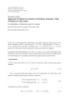
EURASIP Journal on Advances in Signal Processing 7 100 5000 0 Fc1 (Vs−1 ) V2 (V) −100 0 −200 −300 −5000 −20 −10 −20 −10 0 10 20 30 40 50 0 10 20 30 40 50 Vin (V) Vin (V) (a) (b) ×104 15 10 Fc2 (Vs−1 ) 5 0 −5 −20 −10 0 10 20 30 40 50 Vin (V) Vc1,2 : 0 V, 300 V Vc1,2 : 5 V, 200 V Vc1,2 : 5 V, 300 V Vc1,2 : 0 V, 100 V Vc1,2 : 5 V, 100 V Vc1,2 : 0 V, 200 V (c) Figure 5: Approximating functions for the simulation of the system (12)—output function (a), capacitor C1 up-date (b) and capacitor C2 update (c) functions. ×104 8 400 6 200 Fc1 (Vs−1 ) Vout (V) 4 0 2 −200 0 −2 −400 −20 −10 −20 −10 0 10 20 30 40 50 0 10 20 30 40 50 Vin (V) Vin (V) Vc 1 : 0 V Vc1 : 300 V Vc1 : 100 V Vc1 : 400 V Vc1 : 200 V (b) (a) Figure 6: Approximating functions for the simulation of the system (12)—output function (a) and capacitor C2 update function (b). the algorithms were tested with an E-chord guitar riﬀ the Newton method was 1 × 10−5 . The number of iteration was computed from the whole signal (5 s, 240 × 103 samples). with maximal amplitude around 200 mV. The whole circuit simulation required 2.79 iterations on average and 100 The computational complexity of algorithms based on iterations at the most. In the case of the simulation using approximations is shown in Table 5. There are available block decomposition, the average numbers of iterations were results for the whole preamp simulation as well as for the i1 = 2.1294, i2 = 2.4149, i3 = 2.6806 and maximal numbers blockwise simulation. The numbers were computed from (25) and (26) where diﬀerent types of approximation of of iterations were i1 = 4, i2 = 5, i3 = 100 for each block, appropriate order N from Section 4 were used. Similarly, the respectively. The number of iteration of individual block diﬀers because each block processes a diﬀerent signal. The whole system can be approximated by order of approxima- tion N = 5, because the whole circuit contains 4 capacitors. maximum number of iteration was 100 and the error limit of
8 EURASIP Journal on Advances in Signal Processing Table 5: Computational complexity comparison of simulations However, the whole circuit simulation was not implemented based on approximations—number of operations. due to complex approximating functions and also the look- up table size would be huge. Simulation Linear Spline Spline As the results available in Tables 4 and 5 have shown, type interpretation Interpertation Approx the algorithms based on approximation oﬀer constant 9.38 × 102 5.28 × 104 9.53 × 102 Whole computational complexity, which is also much lower than 2.06 × 102 2.58 × 103 2.51 × 102 By blocks at the algorithms based on the Newton method. The linear interpolation has the lowest computational complexity. However, due to higher memory demands it is not suitable Table 6: Errors for simulation from Figure 8. The plate voltage and therefore the spline approximation was chosen as the signal errors are displayed. best method. — V p1 V p2 6.27 × 10−4 2.38 × 10−1 Max [V] 1.13 × 10−5 5.70 × 10−3 Mean [V] 6. Simulation Results 1.05 × 10−7 2.54 × 10−4 var [V] The algorithm was implemented in C++ language as the — V p3 V p4 VST plug-in eﬀect and then tested in realtime. It was tested 2.12 × 10−1 Max [V] 1.99 with a 2.66 GHz i7 Intel Mac with 4 GB RAM at a sampling 1.01 × 10−2 6.20 × 10−3 Mean [V] frequency of 48 kHz using an external audio interface M- 1.07 × 10−3 0.13 × 10−3 var [V] Audio Fast Track Pro with the ASIO buﬀer size 128 samples. If no oversampling was used, the CPU load was around 3%. To reduce aliasing distortion, 4-x oversampling was imple- Table 7: Harmonics comparison from Figure 11. The magnitudes mented. Polyphase FIR interpolation and decimation was are related to the ﬁrst harmonic. used. The CPU load with 4-x oversampling was around 6%. — 2 3 4 5 6 The proposed algorithm was then tested with diﬀerent input −35.1 −10.0 −36.1 −14.7 −37.7 Meas. [dB] signals including a sinusoid signal at diﬀerent frequencies −27.4 −9.8 −28.3 −14.7 −29.5 Sim. [dB] and amplitudes (including frequencies close to the Nyquist Diﬀ. [dB] 7.6 0.2 7.7 0.1 8.2 frequency), logarithmic sweep signal (see Figure 7) and also a real guitar signal. All the performed simulations were stable even if no oversampling was used and the amplitude of the testing signal was around hundreds of volts at the input of the digital simulation was made using sinusoid signal because a third block. Comparison between the simulation of whole harmonic signal generator was used as a signal source for preamp using the Newton method and the simulation based the guitar preamp. The output signal was recorded using on the spline approximation is plotted in Figure 8. Time soundcard. The input harmonic signal had an amplitude of diﬀerence signals are normalized to the maximal value of the 150 mV and a frequency of 1 kHz. Measured and simulated output signal. time-domain signals are shown in Figure 10. Most of the The error values, such as maximal and average error, are errors occur on transients, but the testing preamp was also expressed in Table 6. The maximal error is around 2 V. extremely noisy, and therefore it is very hard to determine An ampliﬁcation of the preamp is approximately 1.84 × 104 the deviation of the simulation. The spectrum of the signals is and measured level of noise at the output of the preamp shown in Figure 11. The rectangular window with a length of without connected guitar is approximately 4.7 Vpp and with a hundredfold of the signal period (48 samples at a sampling connected guitar it is approximately 32 Vpp (these high values frequency of 48 kHz) was used to minimize spectrum leak- are caused by extremely high ampliﬁcation, normally, the age. The measured preamp was homemade and it was not ampliﬁcation is lower). Therefore the error can be masked. In shielded. Therefore, intermodulation distortion components places with the maximal error, the Newton method reached occur in measured spectrum. Table 7 shows magnitudes the maximal number of iterations (100), and therefore the of the higher harmonic components related to the ﬁrst error is caused partly by the approximation and partly by the harmonic. The error between measurement and simulation Newton method. is shown as well. The odd harmonics were almost the The circuit was also simulated with a reduced power same, but the even harmonic were higher in the simulation. supply voltage to 261 V and the results were compared to However, this deviation can be caused by the tube model, a real home-made guitar preamp connected according to because the same simulation results were obtained using the the circuit schematic in Figure 1 with the reduced power numerical solution of the whole circuit. The general model supply. Firstly, the simulations using Newton method and of a 12ax7 tube was used in the simulation but the real tubes have diﬀerent properties—there are many diﬀerent types approximations were compared in Figure 9. The error was of 12ax7 tube and also the same type can diﬀer because approximately the same as in Figure 8—the maximum error increased from 2 V to 3.5 V but the average error of a manufacturer’s tolerance. In order to get an accurate decreased from 6.20 × 10−3 to 4.50 × 10−3 V. The relative simulation, the general tube model must be tuned according error in Figure 9 is higher due to lower power supply. to the used tubes. However, it requires a measurement of the The comparison between the output of real circuit and its transfer functions of the used tubes.
EURASIP Journal on Advances in Signal Processing 9 20000 20000 10000 10000 f (Hz) f (Hz) 1000 1000 100 100 0 0.5 1 1.5 2 2.5 3 0 0.5 1 1.5 2 2.5 3 t (s) t (s) (a) (b) 20000 20000 10000 10000 f (Hz) f (Hz) 1000 1000 100 100 0 0.5 1 1.5 2 2.5 3 0 0.5 1 1.5 2 2.5 3 t (s) t (s) (c) (d) Figure 7: Simulation results for a logarithmic sweep signal. The plate voltage signals p1 , p2 , p3 , and p4 are displayed. The 32-x oversampling was used to reduce aliasing. U p1 error (%) U p1 error (V) U p2 error (%) U p2 error (V) 0 0.01 0.4 0.02 0.2 0.05 0.01 0.005 0.1 0 0 0 0 500 1000 1500 0 500 1000 1500 t (ms) t (ms) (a) (b) U p4 error (%) U p3 error (%) U p4 error (V) U p3 error (V) 0.5 2 0 0.4 0.2 0.05 0 0.1 0 0 0 500 1000 1500 0 500 1000 1500 t (ms) t (ms) (c) (d) Figure 8: Comparison between simulation results using numerical solution and using approximations for a part of a real guitar riﬀ. Only the error signals are displayed. U p2 error (%) U p1 error (%) U p2 error (V) 0.2 0.04 0.01 U p1 error (V) 0.04 0.15 0.03 0.1 0.02 0.005 0.02 0.05 0.01 0 0 0 0 0 2 4 6 8 10 12 14 16 18 0 2 4 6 8 10 12 14 16 18 ×10 3 ×10 3 t (ms) t (ms) (a) (b) U p3 error (%) U p4 error (V) U p3 error (V) U p4 error (%) 1 0.1 4 0.4 0.5 2 0.05 0.2 0 0 0 0 0 2 4 6 8 10 12 14 16 18 0 2 4 6 8 10 12 14 16 18 ×10 3 ×10 3 t (ms) t (ms) (c) (d) Figure 9: Comparison between simulation results using numerical solution and using approximations for the reduced power supply voltage.
10 EURASIP Journal on Advances in Signal Processing 150 200 140 100 Uout (V) 130 Uout (V) 0 120 −100 110 −200 100 0.9 1 1.1 1.2 1.3 1.4 0 0.002 0.004 0.006 0.008 0.01 t (ms) t (ms) ×10−3 Measured Simulated (b) (a) Figure 10: Comparison between measured and simulated preamp. The input voltage was sinewave signal with an amplitude of 150 mV and a frequency of 1 kHz. 40 40 M (dB) M (dB) 20 20 0 0 0 0.5 1 1.5 2 2.5 0 0.5 1 1.5 2 2.5 ×104 f (Hz) ×104 f (Hz) Measured Simulated by blocks (a) (b) 40 M (dB) 20 0 0 0.5 1 1.5 2 2.5 ×104 f (Hz) Simulated (c) Figure 11: Spectrum comparison between measured and simulated preamps. diﬀers in even harmonics. This was probably caused by 7. Conclusion the tube models that were used in simulation, because the In this paper, real-time simulation of a guitar tube ampliﬁer numerical solution of the whole circuit and simulation using using approximations is proposed. The approximation of the approximation were almost the same. Diﬀerent ampliﬁcation solution of diﬀerential equations oﬀers suﬃcient accuracy factor of the tube model can cause the bias shift resulting in diﬀerent results. of the simulation while the computational cost is relatively low. The approximations are used together with the modiﬁed The major advantage of the proposed algorithm is con- blockwise method that allows further reduction of the stant computational complexity and also the computational computational complexity. The blockwise method has been complexity is independent from the number of nonlinear tested and it gives almost the same results as the simulation functions in the simulated circuit or from the number of of the whole circuit. The results of the ampliﬁer simulation circuit nodes. It depends only on the number of accu- were compared with the measurement of the real ampliﬁer mulation elements. However, this is also disadvantageous, because the implementation of approximating functions is and the results show that the quite good accuracy of the quite complicated. Therefore, practically, the number of simulation can be obtained. However, the compared signals
EURASIP Journal on Advances in Signal Processing 11 on Digital Audio Eﬀects (DAFx ’10), Graz, Austria, September accumulation elements is bounded. Nevertheless, this disad- 2010. vantage is compensated for by using the blockwise method. Compared to other methods, this method oﬀers quite simple [12] D. T. Yeh, J. S. Abel, A. Vladimirescu, and J. O. Smith, “Nu- merical methods for simulation of guitar distortion circuits,” implementation, because it is derived directly from circuit Computer Music Journal, vol. 32, no. 2, pp. 23–42, 2008. equations. Thus, no transformations are necessary and the [13] J. Macak and J. Schimmel, “Real-time guitar tube ampliﬁer implementation should be faster. However, comparison with simulation using approximation of diﬀerential equations,” in other methods has not been done yet and therefore this will Proceedings of the 13th International Conference on Digital be the next work. Audio Eﬀects (DAFx ’10), Graz, Austria, September 2010. [14] J. Macak, “Modiﬁed blockwise method for simulation of Acknowledgment guitar tube ampliﬁers,” in Proceedings of 33nd International Conference Telecommunications and Signal Processing (TSP This paper was prepared within the framework of project ’10), pp. 1–4, Vienna, Austria, August 2010. no. FR-TI1/495 of the Ministry of Industry and Trade of the [15] N. Koren, “Improved vacuum tube models for SPICE sim- Czech Republic. ulations,” 2003, http://www.normankoren.com/Audio/Tube- modspice article.html. References [16] Spectrum Software, Micro-Cap 10, Spectrum Software, Sun- nyvale, Calif, USA, 2010. [1] J. Pakarinen and D. T. Yeh, “A review of digital techniques [17] J. M. Miller, “Dependence of the input impedance of a three- for modeling vacuum-tube guitar ampliﬁers,” Computer Music electrode vacuum tube upon the load in the plate circuit,” Journal, vol. 33, no. 2, pp. 85–100, 2009. in Scientiﬁc Papers of the Bureau of Standards, pp. 367–385, [2] D. T. Yeh, J. S. Abel, and J. O. Smith, “Simulation of the diode Washington, DC, USA, September 1920. limiter in guitar distortion circuits by numerical solution of [18] W. H. Press, S. A. Teukolsky, W. T. Vetterling, and B. P. ordinary diﬀerential equations,” in Proceedings of the Digital Flannery, Numerical Recipes in C, Cambridge University Press, Audio Eﬀects (DAFx ’07), pp. 197–204, Bordeaux, France, Cambridge, UK, 2nd edition, 1992. September 2007. U. Z¨ Lzer, DAFX—Digital Audio Eﬀects, John Wiley & Sons, [19] o [3] D. T. Yeh, J. S. Abel, and J. O. Smith, “Simpliﬁed, physically- New York, NY, USA, 1st edition, 2002. informed models of distortion and overdrive guitar eﬀects [20] C. de Boor, A Practical Guide to Splines, Springer, New York, pedal,” in Proceedings of the Digital Audio Eﬀects (DAFx ’07), NY, USA, 1st edition, 2001. pp. 189–196, Bordeaux, France, September 2007. [4] A. Novak, L. Simon, and P. Lotton, “Analysis, synthesis, and classiﬁcation of nonlinear systems using synchronized swept- sine method for audio eﬀects,” EURASIP Journal on Advances in Signal Processing, vol. 2010, Article ID 793816, 8 pages, 2010. [5] J. Pakarinen, M. Tikander, and M. Karjalainen, “Wave digital modeling of the output chain of a vacuum-tube ampliﬁer,” in Proceedings of the International Conference on Digital Audio Eﬀects (DAFx ’09), pp. 1–4, Como, Italy, September 2009. [6] M. Karjalainen and J. Pakarinen, “Wave digital simulation of a vacuum-tube ampliﬁer,” in Proceedings of the IEEE Inter- national Conference on Acoustics, Speech and Signal Processing (ICASSP ’06), pp. 153–156, Toulouse, France, May 2006. [7] J. Pakarinen and M. Karjalainen, “Enhanced wave digital triode model for real-time tube ampliﬁer emulation,” IEEE Transactions on Audio, Speech and Language Processing, vol. 18, no. 4, pp. 738–746, 2010. [8] D. T. Yeh and J. O. Smith, “Simulating guitar distortion circuits using wave digital and nonlinear state-space formulations,” in Proceedings of the Digital Audio Eﬀects (DAFx ’08), pp. 19–26, Espoo, Finland, September 2008. [9] K. Dempwolf, M. Holters, and U. Z¨ Lzer, “Disceetization o of parametric analog circuits for realtime simulations,” in Proceedings of the 13th International Conference on Digital Audio Eﬀects (DAFx ’10), Graz, Austria, September 2010. [10] D. T. Yeh, J. S. Abel, and J. O. Smith, “Automated physical modeling of nonlinear audio circuits for real-time audio eﬀectspart I: theoretical development,” IEEE Transactions on Audio, Speech and Language Processing, vol. 18, no. 4, pp. 728– 737, 2010. [11] I. Cohen and T. Helie, “Real-time simulation of a guitar power ampliﬁer,” in Proceedings of the 13th International Conference