


Lecture Advanced Econometrics (Part II) - Chapter 13: Generalized method of moments (GMM)
lượt xem 5
download
 Download
Vui lòng tải xuống để xem tài liệu đầy đủ
Download
Vui lòng tải xuống để xem tài liệu đầy đủ
Lecture "Advanced Econometrics (Part II) - Chapter 13: Generalized method of moments (GMM)" presentation of content: Orthogonality condition, method of moments, generalized method of moments, GMM and other estimators in the linear models, the advantages of GMM estimator, GMM estimation procedure.
Bình luận(0) Đăng nhập để gửi bình luận!
Nội dung Text: Lecture Advanced Econometrics (Part II) - Chapter 13: Generalized method of moments (GMM)
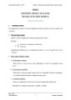
- Advanced Econometrics Chapter 13: Generalized Method of Moments Chapter 13 GENERALIZED METHOD OF MOMENTS (GMM) I. ORTHOGONALITY CONDITION: The classical model: =Y X β + ε ( n×1) ( n×k ) ( k ×1) ( n×1) (1) E (ε X ) = 0 (2) E (εε / X ) = σ 2 I (3) X and ε are generated independently. If E (ε i X i ) = 0 then (for equation= i: Yi X β + εi ) (1×k ) ( k ×1) E ( X iε i ) = E X i E ( X iε i X i ) = E X i E (ε i X i ) X i 0 X i [ 0. X i ] = E= 0 ( k ×1) → Orthogonality condition. ( ) E X i/ − E ( X i/ ) ( ε i − E (ε i ) ) Note: Cov( X i/ , ε i ) = ( = E X i/ − E ( X i/ ) ε i ) ( ) = E X i/ ε i − E ( X i/ ) E (ε i ) 0 / X i εi = E= 0 if E (ε X ) = 0 ( k ×1) (1×1) ( k ×1) So for the classical model: E X i/ ε i = 0 ( k ×1) (1×1) ( k ×1) Nam T. Hoang UNE Business School 1 University of New England
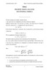
- Advanced Econometrics Chapter 13: Generalized Method of Moments II. METHOD OF MOMENTS Method of moments involves replacing the population moments by the sample moment. Example 1: For the classical model: Population : E ( X i/ε i ) = 0 → E X i/ (Yi − X i β ) = 0 ( k ×1) population moment Sample moment of this: 1 n / 1 / ∑ βˆ ) X i (Yi − X i= X (Y − X βˆ ) n ( k ×n ) n i =1 ( k ×1) 1×1 n×1 ( k ×1) Moment function: A function that depends on observable random variables and unknown parameters and that has zero expectation in the population when evaluated at the true parameter. m( β ) - moment function – can be linear or non-linear. β is a vector of unknown parameters. ( k ×1) E[m( β )] = 0 population moment. Method of moments involves replacing the population moments by the sample moment. Example 1: For the classical linear regression model: The moment function: X i/ ε i = m( β ) The population function: E ( X i/ ε i ) = 0 E [ m( β )= ] E X i/ (Yi − X i β )= 0 ( k ×1) The sample moment of E ( X i ε i ) is 1 n / 1 / ∑ βˆ ) X i (Yi − X i= X (Y − X βˆ ) n ( k ×n ) n i =1 ( k ×1) 1×1 n×1 ( k ×1) Replacing sample moments for population moments: Nam T. Hoang UNE Business School 2 University of New England
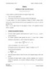
- Advanced Econometrics Chapter 13: Generalized Method of Moments 1 / n ( X Y − X βˆ = 0 ) X /Y − X / X βˆ = 0 X / X βˆ = X /Y =βˆMOM (= X / X ) −1 X /Y βˆOLS Example 2: If X i are endogenous → Cov( X i/ , ε ) ≠ 0 (1×k ) Suppose Z i = ( Z1i Z 2i Z Li ) is a vector of instrumental variables for X i (1× L ) (1×k ) Zi satisfies: E (ε i Z= i ) 0 → E ( Z i/ε i ) = 0 and Cov ( Z i/ε i ) = 0 (1× L ) ( L×1) ( L×1) We have: E ( Z i/ ε i ) = 0 ( L×1) (1×1) ( L×1) E Z i/ (Yi − X i β ) = 0 ( L×1) population moment The sample moment for E Z i/ (Yi − X i β ) is 1 n / ∑ Zi Yi − X i βˆ n i =1 ( ) 1 = Z / Y − X βˆ n ( L ×n ) ( k ×1) ( n×1) ( L×1) Replacing sample moments for population moments: 1 / Z Y − X βˆ = 0 (*) n ( L ×n ) ( k ×1) ( L ×1) ( n×1) a) If L < k (*) has no solution b) If L = k exact identified. Nam T. Hoang UNE Business School 3 University of New England
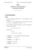
- Advanced Econometrics Chapter 13: Generalized Method of Moments Z / Y − X βˆ = 0 ( L ×n ) ( n×k ) ( k ×1) ( k ×1) Z / X βˆ = Z /Y βˆMOM (= = Z / X ) −1 Z /Y βˆIV c) If L > k → k parameters, L equations → There is NO unique solution because of "too many" equations → GMM. III. GENERALIZED METHOD OF MOMENTS: 1. The general case: / ( βˆ ) is the sample moment of the population moment E [m( β )] = 0 Denote: m Method of moments: βˆ1 βˆ m/ ( βˆ ) = 0 βˆ = 2 ( k ×1) ( L×1) ( L×1) βˆk a) If L < k: no solution for βˆ b) If L = k: unique solution for βˆ as m/ ( βˆ ) = 0 ( k ×1) ( L×1) ( L×1) c) If L > k, how do we estimate β ? Hausen (1982) suggested that instead of solving the equations for βˆ / ( βˆ ) = ( L× m 0 1) ( k ×1) We solve the minimum problem: / min m/ ( βˆ ) ( W m/ ( βˆ ) (**) βˆ L× L ) (1× L ) ( L×1) Where W is any positive definite matrix that may depend on the data. Note: If X is a positive definite matrix then for any vector a = ( a1 a2 an ) ( n ×n ) a/ X a > 0 (1×n ) ( n×n ) (1×n ) Nam T. Hoang UNE Business School 4 University of New England
- Advanced Econometrics Chapter 13: Generalized Method of Moments βˆ that minimize (**) is called generalized method of moments (GMM) estimator of βˆ , denote βˆGMM . Hausen (1982) showed that βˆGMM from (**) is a consistent estimator of β. p lim βˆGMM = β n →∞ ( k ×1) Problem here: What is the best W to use ? - Hansen (1982) indicated: −1 W = VarCov ( n m( βˆ )) ( L× L ) - With this W, βˆGMM is efficient → has the smallest variance: 1 −1 VarCov ( βˆGMM ) = G /WG n ∂m( βˆ ) where: G = p lim ( L ×k ) ∂βˆ / ( ) 1 −1 −1 VarCov βˆGMM = G /WG / G /W VarCov n m( βˆ ) WG G /WG n 2. The linear model: 1 n ∑ n i =1 Z i/ (Yi − X i β ) = m/ ( β ) The sample moment becomes: / n n = min βˆ ∑ i 1= Z i / ( Yi − X i β ) W ∑ ( L× L ) i 1 Z i/ (Yi − X i β ) (1× L ) ( L×1) First- order condition: / n / n ∑ ( L×i1) (1×ki ) ( L×L ) ∑ Z i (Yi − X i β ) = / Z X W 0 = i 1= i 1 ( k ×1) (1× L ) ( L×1) k equations: ( Z X ) W ( Z Y − Z X βˆ ) = / → / / 0 / ( Z X ) W .Z X βˆ ( Z X ) W .Z Y = / / → / / / / Nam T. Hoang UNE Business School 5 University of New England
- Advanced Econometrics Chapter 13: Generalized Method of Moments −1 → βˆGMM =( Z / X ) / W .Z / X ( Z / X ) / W .Z /Y For the linear regression model: −1 / βˆGMM = ( X / Z ) W ( Z / X ) ( X Z ) (W ( Z /Y ) ( k ×1) ( k ×L ) ( L×L ) ( L×1) ( k ×L ) L×L ) ( L×1) IV. GMM AND OTHER ESTIMATORS IN THE LINEAR MODELS: 1. Notice that if L = k (exact identified) then X / Z is a square matrix ( k × k ) so that: ( X / Z ) .W . ( Z / X ) = ( Z / X ) W −1. ( X / Z ) −1 −1 −1 βˆGMM = ( Z / X ) (Z Y ) −1 / and which is the IV estimator → The IV estimator is a special case of the GMM estimator. (X X ) (X Y ) −1 2. If Z = X then βˆGMM = βˆ= OLS / / 3. If L > k over-identification, the choice of matrix W is important. W is called weight matrix. βˆGMM is consistent for any W positive definite. The choice of W will affect the variance of βˆGMM → We could choose W such that Var ( βˆGMM ) is the smallest → efficient estimator. 4. If W = ( Z / Z ) −1 then: −1 βˆGMM = ( X / Z )( Z / Z ) ( Z / X ) ( X / Z )( Z / Z ) ( Z /Y ) −1 −1 which is the 2SLS estimator is also a special case of the GMM estimator. 5. From Hausen (1982), the optimal W in the case of linear model is: −1 1 E ( Z i/ε i ε i/ Z i ) 1 −1 W = Z / ΣZ = n n −1 W = VarCov ( Z i/ε i ) 1 n Nam T. Hoang UNE Business School 6 University of New England
- Advanced Econometrics Chapter 13: Generalized Method of Moments 6. The next problem is to estimate W: a) If no heteroskedasticity and no autocorrelation: −1 −1 1 n W = σˆ ε2 ∑ ( Z i/ Z i ) 1 = σˆ ε2 ( Z / Z ) n i =1 n −1 βˆGMM = ( X / Z )( Z / Z ) ( Z / X ) ( X / Z )( Z / Z ) ( Z /Y ) −1 −1 We get the 2SLS estimator → there is no different between βˆ2 SLS and βˆGMM in the case of no heteroskedasticity and no autocorrelation. b) If there is heteroskedasticity in the error terms (but no autocorrelation) in unknown forms. −1 1 n Wˆ = ∑ ( ei2 Z i/ Z i ) (White's estimator) → efficient gain over βˆ2 SLS . n i =1 c) If there are both heteroskedasticity and autocorrelation in unknown forms, use: Wˆ = Newey - West estimator) . −1 1 = Wˆ Z / ΣZ n −1 1 n ∑ ( Z i Z i ei ) + ∑ ∑ w j ei ei − j ( Z i Z i − j + Z i − j Z i ) L n Wˆ = / 2 / / n i= 1 j = 1 i = j +1 j → efficient gain over β 2 SLS ˆ wj = 1 − L +1 Notes: Σ = E (ε iε i/ ) if heteroskedasticity and autocorrelation forms are known σ 2 = f ( X i ) EX: i then Σ = E (ε iε i/ ) can be consistently estimated and we =ε t ρε t −1 + ut could perform GLS to get the efficient estimators βˆGLS (using instrumental variables), GMM is not necessary here. Usually the form of autocorrelation and heteroskedasticity are not known → GMM estimator is an important improvement in these cases. Nam T. Hoang UNE Business School 7 University of New England
- Advanced Econometrics Chapter 13: Generalized Method of Moments V. GMM ESTIMATION PROCEDURE: Step 1: Use W = I or W = ( Z / Z ) −1 to obtain a consistent estimator of β. Then estimate Wˆ by White's procedure (heteroskedasticity case) or Newey-West procedure (general case). Step 2: Use the estimated Wˆ to compute the GMM estimator: βˆGMM = ( X / Z ) Wˆ ( Z / X ) ( X / Z ) Wˆ ( Z /Y ) −1 Note: We always need to construct Wˆ in the first step. VI. THE ADVANTAGES OF GMM ESTIMATOR: 1. If we don't know the form/patent of heteroskedasticity or autocorrelation → correct by Robust standard error (White or Newey-West) → stuck with inefficient estimators. 2. 2-SLS estimator is consistent but still inefficient if error terms are correlated/ heteroskedasticity. 3. GMM brings efficient estimator in the case of unknown heteroskedasticity and autocorrelation forms/ correct standard errors also. Potential drawbacks: 1. Definition of the weight matrix W for the first is arbitrary, different choices will lead to different point estimates in the second step. One possible remedy is to not stop after iterations but continue to update the weight matrix W until convergence has been achieved. This estimator can be obtained by using the "cue" (continuously updated estimators) option within ivreg 2 2. Inference problem because the optimal weight matrix is estimated → can lead to sometime downward bias in the estimated standard errors for GMM estimator. Nam T. Hoang UNE Business School 8 University of New England
- Advanced Econometrics Chapter 13: Generalized Method of Moments VII. VARIANCE OF THE GMM ESTIMATOR FOR LINEAR MODELS: ( ) Note: VarCov βˆGMM = ( X / Z ) Wˆ ( Z / X ) 1 −1 1 −1 n →∞ → Q X / ZWˆ .QZ / X n n n→∞ → 0 → consistency. ( ) ( → N 0, Q X / ZWQ ) so that βˆ −1 n βˆGMM − β L ˆ / GMM is consistent estimator. Z X ( ) Estimated: VarCov βˆGMM = n ( X / Z ) Wˆ ( Z / X ) −1 In practice Wˆ is noise, since the residual in the first step are affected by sampling error. The upshot is that step 2 standard errors tend to be too good. Methods now exist that enable you to correct for sampling error in the first step (Windmeijer procedure). VIII. SPECIFICATION TESTS WITH GMM: βˆGMM R : Restricted estimator (under constraints). βˆGMM : Unrestricted estimator (no constraints). n / n n n / ∑ i i ε 2∑ i i ε − ∑ i i 2 ∑ Zi ε i / n χ q ε J Z ˆ ( R )Wˆ Z / ˆ ( R ) Z / ˆ Wˆ ˆ 2 = i 1 =i 1 =i 1 =i 1 q: number of restrictions. Nam T. Hoang UNE Business School 9 University of New England
CÓ THỂ BẠN MUỐN DOWNLOAD
-
Lecture Advanced Econometrics (Part II) - Chapter 3: Discrete choice analysis - Binary outcome models
 18 p |
  67
|
67
|  6
6
-
Lecture Advanced Econometrics (Part II) - Chapter 4: Discrete choice analysis - Multinomial models
13 p | 78
| 4
-

Lecture Advanced Econometrics (Part II) - Chapter 5: Limited dependent variable models - Truncation, censoring (tobit) and sample selection
13 p | 62
| 4
-
Lecture Advanced Econometrics (Part II) - Chapter 6: Models for count data
7 p | 86
| 4
-
Lecture Advanced Econometrics (Part II) - Chapter 1: Review of least squares & likelihood methods
6 p | 68
| 3
-
Lecture Advanced Econometrics (Part II) - Chapter 2: Hypothesis testing
7 p | 57
| 3


Chịu trách nhiệm nội dung:
Nguyễn Công Hà - Giám đốc Công ty TNHH TÀI LIỆU TRỰC TUYẾN VI NA
LIÊN HỆ
Địa chỉ: P402, 54A Nơ Trang Long, Phường 14, Q.Bình Thạnh, TP.HCM
Hotline: 093 303 0098
Email: support@tailieu.vn
Giấy phép Mạng Xã Hội số: 670/GP-BTTTT cấp ngày 30/11/2015 Copyright © 2022-2032 TaiLieu.VN. All rights reserved.

