


Mạng Nơ-ron hồi quy
lượt xem 2
download
 Download
Vui lòng tải xuống để xem tài liệu đầy đủ
Download
Vui lòng tải xuống để xem tài liệu đầy đủ
RNN có khả năng nhớ các thông tin được tính toán trước. Gần đây, mạng LSTM đang được chú ý và sử dụng khá phổ biến. Về cơ bản mô hình của LSTM không khác mô hình truyền thống của RNN, nhưng chúng sử dụng hàm tính toán khác ở các trạng thái ẩn. Vì vậy mà ta có thể truy xuất được quan hệ của các từ phụ thuộc xa nhau rất hiệu quả. Việc ứng dụng LSTM sẽ được giới thiệu ở bài báo sau. Mời các bạn cùng tham khảo chi tiết nội dung bài viết!
Bình luận(0) Đăng nhập để gửi bình luận!
CÓ THỂ BẠN MUỐN DOWNLOAD


Chịu trách nhiệm nội dung:
Nguyễn Công Hà - Giám đốc Công ty TNHH TÀI LIỆU TRỰC TUYẾN VI NA
LIÊN HỆ
Địa chỉ: P402, 54A Nơ Trang Long, Phường 14, Q.Bình Thạnh, TP.HCM
Hotline: 093 303 0098
Email: support@tailieu.vn
Giấy phép Mạng Xã Hội số: 670/GP-BTTTT cấp ngày 30/11/2015 Copyright © 2022-2032 TaiLieu.VN. All rights reserved.

