Tối ưu hóa viễn thông và thích nghi Kỹ thuật Heuristic P19

Chia sẻ: Tien Van Van | Ngày: | Loại File: PDF | Số trang:15

Thêm vào BST

Báo xấu

78
lượt xem 5
download

Download Vui lòng tải xuống để xem tài liệu đầy đủ

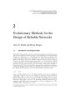
Channel Assignment Problems (CAPs) occur in the design of cellular mobile telecommunication systems (Jordan, 1996; Katzela and Naghshineh, 1996; MacDonald, 1979); such systems typically divide the geographical region to be serviced into a set of cells, each containing a base station. The available radio frequency spectrum is divided into a set of disjoint channels; these must be assigned to the base stations to meet the expected demand of each cell and to avoid electromagnetic interference during calls....

Chủ đề:

Bình luận(0) Đăng nhập để gửi bình luận!

Lưu

Nội dung Text: Tối ưu hóa viễn thông và thích nghi Kỹ thuật Heuristic P19

Telecommunications Optimization: Heuristic and Adaptive Techniques. Edited by David W. Corne, Martin J. Oates, George D. Smith Copyright © 2000 John Wiley & Sons Ltd ISBNs: 0-471-98855-3 (Hardback); 0-470-84163X (Electronic) 19 An Effective Genetic Algorithm for the Fixed Channel Assignment Problem George D. Smith, Jason C.W. Debuse, Michael D. Ryan and Iain M. Whittley 19.1 Introduction Channel Assignment Problems (CAPs) occur in the design of cellular mobile telecommunication systems (Jordan, 1996; Katzela and Naghshineh, 1996; MacDonald, 1979); such systems typically divide the geographical region to be serviced into a set of cells, each containing a base station. The available radio frequency spectrum is divided into a set of disjoint channels; these must be assigned to the base stations to meet the expected demand of each cell and to avoid electromagnetic interference during calls. There are many different approaches to assigning channels to these base stations to achieve these objectives. The most commonly used technique is the Fixed Channel Assignment (FCA) scheme, in which channels are assigned to each base station as part of the design stage and are essentially fixed in that no changes can be made to the set of channels available for a cell. There are also Dynamic Channel Assignment (DCA) schemes, in which all of the available channels are stored in a common pool; each new call that arrives in a cell is assigned a channel from this pool as long as it does not interfere with existing channels that are currently in use; see Katzela and Naghshineh (1996). There are also hybrids of FCA and DCA schemes as well as other variants, such as Channel Borrowing methods. It has been shown that DCA schemes beat FCA schemes, except under Telecommunications Optimization: Heuristic and Adaptive Techniques, edited by D. Corne, M.J. Oates and G.D. Smith © 2000 John Wiley & Sons, Ltd
358 Telecommunications Optimization: Heuristic and Adaptive Techniques conditions of heavy traffic load (Raymond, 1991). Since networks are under increasing pressure to meet ever increasing demand, an effective solution to the FCA problem is therefore extremely desirable. The algorithms presented in this paper have been developed for the FCA problem. Customers of the network rely on the base station of the cell in which they are situated to provide them with a channel through which they can make a call. In solving the FCA problem, network designers must allocate channels to all the cells in the network as efficiently as possible so that the expected demand of each cell is satisfied and the number of violations of Electro-Magnetic Compatibility constraints (EMCs) in the network is minimised. This paper considers three types of electro-magnetic constraints: • Co-channel (CCC); some pairs of cells may not be assigned the same channel. • Adjacent channel (ACC); some pairs of cells may not be assigned channels which are adjacent in the electromagnetic spectrum. • Co-site (CSC); channels assigned to the same cell must be separated by a minimum frequency distance. These and further constraints may be described within a compatibility matrix C, each element Cij of which represents the minimum separation between channels assigned to cells i and j, see for example Ngo and Li (1998), Funabiki and Takefuji (1992) and Gamst and Rave (1982). In addition to satisfying these interference constraints, solutions may be required to minimise the total number of channels used or the difference between the highest and lowest channel used, to make more efficient use of the electromagnetic spectrum and therefore to allow for future network expansion. Solving instances of the FCA problem is not a trivial exercise. If we consider a simple network that exhibits just one of the constraints described above, the CCCs, then the problem is identical to Graph Colouring. The Graph Colouring problem is known to be NP- Complete, (Garey and Johnson, 1979) and consequently it is very unlikely that a polynomial time algorithm exists that can solve all instances of the FCA problem. There have been many approaches to the solution of the FCA problem, including heuristic techniques such as genetic algorithms (Ngo and Li, 1998; Crisan and Mühlenbein, 1998; Valenzuela et al., 1998; Lai and Coghill, 1996; Cuppini, 1994), simulated annealing (Duque-Antón et al., 1993, Clark and Smith, 1998), local search (Wang and Rushforth, 1996), artificial neural networks (Funabiki and Takefuji, 1992; Kunz, 1991) and various greedy and iterative algorithms (Sivarajan et al., 1989; Box, 1978; Gamst and Rave 1982). Heuristic search techniques tend to adopt one of two strategies to solve the FCA problem: • A direct approach that uses solutions that model the network directly, i.e. they contain information about which channels are assigned to which cells. • An indirect approach whose solutions do not model the network directly. Typically the solutions represents a list of all the channels required to satisfy the demand of the network. Algorithms such as those described by Sivarajan et al. (1989) and Clark and Smith (1998) are used to transform the indirect solutions into real network models that can be used to evaluate the quality of the proposed solutions.
An Effective Genetic Algorithm for the Fixed Channel Assignment Problem 359 Standard genetic algorithms using a direct representation have been found to perform quite poorly on the FCA problem. Cuppini (1994) and Lai and Coghill (1996) attempt to solve only relatively trivial FCA problems. Ngo and Li (1998) successfully apply their GA to more difficult problems but they report run times of over 24 hours for a single run of some of the simpler problem instances. In addition, they also employ a local search algorithm which fires when the GA gets stuck in a local optimum. In short, the literature does not provide much evidence that an efficient and scalable channel assignment system could be based on a standard GA. This chapter describes a genetic algorithm that adopts a direct approach to solving the FCA problem. The GA is unusual in that it is able to utilise partial (or delta) evaluation of solutions, thereby speeding up the search. In addition, we compare the results of the GA with those of a simulated annealing algorithm that uses the same representation and fitness function as the GA, as well as similar neighbourhood move operators. More details of the algorithms and results presented here can be found in Ryan et al. (1999). Details of the representation, fitness function and operators used by the GA and SA are presented in section 19.2, as are some additional enhancements used by the GA. The benchmark problems on which the algorithms have been tested are shown in section 19.3 and experimental results are presented in section 19.4. Finally, a summary of the work is presented in section 19.5, including details of current work using other heuristic algorithms. 19.2 The Hybrid Genetic Algorithm 19.2.1 A Key Feature of the Hybrid GA Designing a genetic algorithm for the FCA problem using a direct approach that will execute in a reasonable amount of time is very difficult. The main obstacle to efficient optimisation of assignments using a traditional genetic algorithm is the expense of evaluating a solution. Complete evaluation of a solution to the FCA problem can be extremely time consuming. Algorithms based on neighbourhood search, such as simulated annealing, can typically bypass this obstacle using delta evaluations. Each new solution created by the neighbourhood search algorithm differs only slightly from its predecessor. Typically the contents of only a single cell are altered. By examining the effects these changes have on the assignment, the fitness of the new solution can be computed by modifying the fitness of its predecessor to reflect these changes. A complete evaluation of the assignment is avoided and huge gains in execution times are possible. Unfortunately, such delta evaluations are difficult to incorporate in the GA paradigm. At each generation a certain proportion of the solutions in a population are subject to crossover. Crossover is a binary operator that combines the genes of two parents in some manner to produce one or more children. The products of a crossover operator can often be quite different from their parents. For example, consider the genetic fix crossover operator employed by Ngo and Li (1998). So long as the two parents are quite different from each other, their children are also likely to be quite dissimilar from both parents. Consequently it is generally impractical to use delta evaluation to compute the fitness of offspring from their parents. After a child has been produced by crossover it must be completely re-evaluated to determine its fitness.
360 Telecommunications Optimization: Heuristic and Adaptive Techniques In the light of this shortcoming, a GA using a simple crossover operator, such as the one employed by Ngo and Li (1998), which requires a large amount of time to evaluate a single solution and which does not appear to guide the population towards a speedy convergence, will be comprehensively outperformed by a local search algorithm, such as simulated annealing, that uses delta evaluations. To be competitive with local search techniques, a GA must utilise operators that allow it either to converge very quickly so few evaluations are required or to explore the search space efficiently using delta evaluations. Section 19.2.3 describes a greedy crossover operator that uses delta evaluations to explore a large number of solutions, cheaply, in an attempt to find the best way to combine two given parents. 19.2.2 Representation The solution representation employed by the hybrid GA is based on the basic representation used by Ngo and Li (1998). Each solution is represented as a bit-string. The bit-string is composed of a number, n, of equal sized segments, where n is the number of cells in the network. Each segment represents the channels that are assigned to a particular cell. Each segment corresponds to a row in Figure 19.1. The size of each segment is equal to the total number of channels available, say m. If a bit is switched on in a cell’s segment, then the channel represented by the bit is allocated to the cell. Each segment is required to have a specific number of bits set at any one time which is equal to the cell’s demand, i.e. the number of channels that must be assigned to this cell. Genetic or other operators must not violate this constraint. The length of a solution is thus equal to the product of the number of cells in the network and the number of channels available, i.e. m times n. Figure 19.1 shows a diagram of the basic representation used. Channel number 1 2 3 ... m-1 m 1 0 1 0 ... 1 0 2 1 0 0 ... 0 1 3 0 0 1 ... 1 0 Cell number ... ... ... ... ... ... ... n-1 1 0 1 ... 0 1 n 0 1 0 ... 1 0 Figure 19.1 Representation of assignment used by the GA and the SA.
An Effective Genetic Algorithm for the Fixed Channel Assignment Problem 361 In fact, Ngo and Li implement a variation of this representation, in which they only store the offsets based on a minimum frequency separation for CSC. Although we have not implemented this extension here, our initialisation procedures and genetic operators ensure that the CSCs are not violated. However, Ngo and Li achieved a significant reduction in the size of the representation and hence the search space through the use of these offsets. This is worth considering for future work. 19.2.3 Crossover A good crossover operator for the FCA problem must create good offspring from its parents quickly. Producing good quality solutions will drive the GA towards convergence in a reasonable number of generations, thus minimising the amount of time the GA will spend evaluating and duplicating solutions. Mutation can be relied on to maintain diversity in the population and prevent the GA from converging too quickly. A research group at the University of Limburg (see Smith et al., 1995) devised such a crossover operator for the Radio Link Frequency Assignment Problem (RFLAP), which proved to be very successful. In essence, they used a local search algorithm to search for the best uniform crossover that could be performed on two parents, to produce one good quality child. Once found, the best crossover was performed and the resulting child took its place in the next generation. Whilst the FCA problem and the RFLAP are significantly different to prevent this particular crossover operator being employed in the former, this research does illustrate how a similar sort of operator may be applied to achieve good results for the FCA problem. The crossover operator employed here uses a greedy algorithm to attempt to find the best combination of genes from two parents to produce one good quality child. The greedy algorithm is seeded with an initial solution consisting of two individual solutions to the FCA problem. The greedy algorithm works by maintaining two solutions. It attempts to optimise only the solution with the best fitness. It achieves this by swapping genetic information between the two solutions. Information can only be swapped between corresponding cells in each of the solutions. When a swap is performed, two channels are selected, one from each solution. The channels are then removed from the solution from which they were originally selected and replaced by the channel chosen from the other solution. The manner in which these swaps are performed is defined by a neighbourhood. The greedy algorithm explores a neighbourhood until it finds an improving swap, i.e. a swap that leads to an improvement in the fitness of the parent targeted for optimisation. When such a swap is found both solutions are modified and the neighbourhood is updated. The greedy algorithm continues to explore the remainder of the neighbourhood searching for more improving moves. The process continues until the entire neighbourhood is explored. At this juncture the solution being optimised is returned as an only child. The neighbourhoods are constructed in the following fashion. Each solution is essentially a sequence of sets, one for each cell in the network. Each set contains a certain number of channels that are assigned to the cell corresponding to this set. Two new sequences of sets are created by performing set subtractions on each of the sets in both parents. These new sequences of sets, referred to as the channel lists, again contain a set for each cell. Each set in channel list 1 contains channels which have been assigned to the cell represented by this set, in the first parent but not to the corresponding cell in the second
362 Telecommunications Optimization: Heuristic and Adaptive Techniques parent and vice versa for channel list 2. The neighbourhood is then constructed from these lists in the following manner: (See Figure 19.2) for each cell c for each channel i in cell c in channel list 1 for each channel j in cell c in channel list 2 Generate move which swaps channels i and j in cell c Since the parents and the channel lists are represented as bit-strings the set subtractions can be efficiently performed as a sequence of ANDs and XORs. The order in which the greedy algorithm explores the moves in the neighbourhood is important. Experimentation has shown that the moves are best explored in a random fashion. Consequently if the crossover operator is applied to the same parents more than once there is no guarantee that the resulting children will be identical. The process of neighbourhood construction is depicted in Figure 19.2. Figure 19.2(a) illustrates the two parents. These are real solutions to Problem 1 as described in section 19.3. This toy problem has only four cells which have demands of 1, 1, 1 and 3 respectively. The cell segments are denoted by the numbers appearing above the solutions. The solutions are not depicted in bit-string form for reasons of clarity. Performing the set subtraction operations described above yields two channel lists that are displayed in Figure 19.2(b). Finally, Figure 19.2(c) depicts all the moves which are generated from the channel lists. These moves define the neighbourhood of all possible moves. Computing the channel lists is a very important part of the crossover operation. It guarantees that each move in the neighbourhood will alter the two solutions, maintained by the crossover operator, in some way. Hence, moves that will not effect the solution we are trying to optimise will not be generated and consequently we will waste no time evaluating the solutions they produce. Interestingly, this aspect of the crossover operator does have an advantageous side effect. As the size of the neighbourhood depends upon the size of the channel lists, the number of solutions evaluated by a crossover operator depends on the similarity between the parents upon which it was invoked. As the population of the GA begins to converge, the crossover operators performs less work and the GA improves its speed. There is one huge advantage of using the neighbourhood described above. Each new solution explored differs only slightly from its predecessor. Consequently, it is entirely practical for the greedy algorithm to employ delta evaluations allowing it to search its neighbourhoods incredibly quickly. So rather than performing one slow evaluation on two solutions as a normal crossover operator would do, it performs quick evaluations on many solutions. The GA can now search the solution space cheaply in the fashion of a local search algorithm. The effect that delta evaluation has on our hybrid GA is dramatic. Some experiments were performed on the first problem set, described in section 19.4, to assess the impact of delta evaluation on the genetic search. The results of these experiments demonstrated that the GA runs about 90 times faster when using delta evaluations. This result illustrates the most important feature of the hybrid GA presented in this paper. Its ability to explore the search space very efficiently allows the GA to produce effective assignments for large and complicated networks in a reasonable amount of time.
An Effective Genetic Algorithm for the Fixed Channel Assignment Problem 363 Cells 0 1 2 3 Solution 1 1 4 7 1 3 9 Solution 2 2 4 8 1 7 10 (a) Moves 0 2 3 Channel List 1 1 7 3 9 Cell 0: (1,2) Cell 2: (7,8) Cell 3: (3,7) , (3,10) Channel List 2 2 8 7 10 (9,7) , (9,10) (b) (c) Figure 19.2 Crossover neighbourhood construction. Finally, relatively low crossover rates of 0.2 and 0.3 have been found to work well with this crossover operator. Due to the greedy nature of the operator, higher crossover rates cause the GA to converge prematurely. 19.2.4 Mutation The nature of the crossover operator described above tends to cause the GA’s population to converge very quickly. Mutation plays an essential role in the hybrid GA by maintaining sufficient diversity in the population, allowing the GA to escape from local optima. Mutation iterates through every bit in a solution and modifies it with a certain probability. If a bit is to be modified, the associated cell is determined. A random bit is then chosen in the same cell that has an opposite value to the original bit. These bits are then swapped and the process continues. The mutation operator cannot simply flip a single bit because this would violate the demand constraints of the cell. A maximum of 100 mutations is permitted per bit-string. Without this limit, mutation would cause the GA to execute very slowly on some of the larger problems.
364 Telecommunications Optimization: Heuristic and Adaptive Techniques 19.2.5 Other GA Mechanisms The hybrid GA is loosely based on Goldberg’s simple GA (Goldberg, 1989). Each generation the individuals in the population are ranked by their fitness. Solutions are selected for further processing using a roulette wheel selection. A certain proportion of solutions for the next generation will be created by the crossover operator described above. The remaining slots in the next generation are filled by reproduction. Mutation is only performed on solutions produced by reproduction. Allowing mutation an opportunity to mutate the products of crossover was found to have a negative impact on the genetic search. Due to the highly epistatic nature of our representation, a single mutation can have a very detrimental impact on the fitness of the solutions produced, after great effort, by the crossover operator. Were mutation applied to all solutions, an excellent assignment produced by crossover could be corrupted completely before it has a chance to enter the next generation. 19.2.6 Fitness The fitness of a solution to the FCA problem is determined by the number of electromagnetic constraints that it violates. It does not include any information as to whether the network demand is satisfied because this constraint is enforced by the representation and the operators used. More precisely, the fitness, F(S), of a solution, S, is given by       n −1 m −1 n −1 p + (Cij −1)  n −1 m −1  p + (Cii −1)  F (S ) = ∑∑ ∑ ∑  S jq Sip + ∑∑ ∑  Siq Sip i =0 p =0  j =0 q = p −(Cij −1)  i =0 p =0  q = p =1   0≤q0 0≤q
An Effective Genetic Algorithm for the Fixed Channel Assignment Problem 365 used by a greedy algorithm which will only perform an improving move. Since we are just optimising the first solution, we do not need to bother considering channels which are assigned to it without violation. Replacing these channels cannot possibly lead to an improvement in the solution as they were not responsible for any interference in the first place. Thus we can omit these channels from the list of channels that can be swapped out of the first solution. Determining which channels in the first channel list are involved in violations is actually quite expensive and involves a partial evaluation of the first solution. However, if it can prevent the crossover operator performing more than a few swaps, some performance gains might be made. It should be noted that, even though delta evaluation is used to recompute the value of solutions after a swap has occurred, the process is still quite slow. Eliminating CSCs Ngo and Li (1998) demonstrate that it is possible to eliminate CSCs completely from the search process for some problems. They achieve this by modifying their representation so that CSCs could not be violated, using a special technique called minimum-separation encoding. While we do not employ this technique, the hybrid GA attempts to employ a similar heuristic without altering the representation. It constructs an initial population that does not contain any CSC violations. This can be achieved by ensuring that for each solution all the channels assigned to a single cell are separated from each other by the CSC frequency separation for that cell. The GA then ensures that neither the crossover nor the mutation operator can perform a swap that can violate a CSC. This heuristic allows us to effectively reduce the size of the search space for certain problems. 19.2.8 Simulated Annealing Finally, in this section, we present the simulated annealing algorithm that was used to contrast the performance of the GA. Simulated annealing (SA) is a modern heuristic search method that is often applied to combinatorial optimisation problems, including the FCA problem; see Duque-Antón (1993). In SA, the search typically starts at a randomly generated solution. At each iteration, a neighbourhood move is suggested, i.e. a change of value for one or more variables, and that move is accepted if it is better. If the suggested move is worse than the current move, it is accepted with a probability that depends on a temperature parameter. Initially, at high temperatures, worse moves are accepted with a relatively high probability, but as the temperature drops, this probability reduces to zero. This basic mechanism reduces the possibility of becoming trapped in a local optimum. The reader is referred to Reeves (1993) for a fuller description of the basic SA algorithm. In this application, the SA uses the same representation employed by the GA; see section 19.2.2. SA does not employ a crossover operator, but instead uses a neighbourhood operator which randomly selects a channel that has been allocated to a cell and attempts to replace it with the best unused channel that is not currently assigned to the cell in question. Delta evaluation is also used in the SA. An initial temperature of 0.1 is used, together with a geometric cooling rate of 0.92 and a temperature step length of 20,000 iterations.
366 Telecommunications Optimization: Heuristic and Adaptive Techniques 19.3 Benchmark Problems All the problems described within this document are defined in terms of the following, as previously described in Funabiki and Takefuji (1992); see also Gamst and Rave (1982). 1. A set of n cells. 2. A set of m channels. 3. An n×n compatibility matrix C as described above. 4. An n element demand vector D, each element di of which represents the number of channels required by cell i. Algorithms designed to solve these problems must generate solutions that completely satisfy the network demand whilst minimising the number of Electro-Magnetic Constraint (EMC) violations. The following objectives must therefore be met by the algorithms applied within this chapter; we will assess their performance in terms of meeting these. • The traffic demand must be met. • The resulting interference must be minimised. • Efficient use should be made of the available spectrum, i.e. we should minimise the number of channels used for an interference-free solution, if possible. 19.3.1 Problem Set 1 Table 19.1 shows some widely used benchmark examples from the literature. Problem 1 is a trivial problem used mostly as illustration, see Sivarajan et al. (1989) and Ngo and Li (1998). Problem 2 is a realistic channel-assignment problem from Kunz (1991). Problems 3 to 11 are a related set of problems taken from a variety of sources, see Ngo and Li (1998) and Wang and Rushforth (1996). Although the problems in this last set all have 21 cells in common, they differ in their traffic demand vector D and the compatibility matrix C; see Wang and Rushforth (1996) for full specifications of these problems. There is one other major difference to the approach that our techniques have. Typically, algorithms will attempt to minimise the number of channels used (or the span) whilst satisfying the traffic demand of each cell and avoiding any interference. In real-world problems, however, one is often given the number of channels that are available as a constraint. The objective, therefore, is to meet the demand and avoid interference by using no more than the number of channels available. If this is not possible, the solution will either not meet the demand or will involve some interference somewhere in the network. For the problems in Problem set 1, the total number of channels available for each problem has been determined by lower bounds (on the number of channels needed) that have been published for these problems in the literature; see Gamst (1986), Funabiki and Takefuji (1992) and Sivarajan et al. (1989). Taking this value, therefore, an interference- free solution to any of the problems in this set will meet all three objectives stated above.
An Effective Genetic Algorithm for the Fixed Channel Assignment Problem 367 Table 19.1 The first set of benchmark problems – Problem set 1. Problem Total cells Total channels Total demand 1 4 11 6 2 25 73 167 3 21 221 470 4 21 309 470 5 21 533 481 6 21 533 481 7 21 381 481 8 21 309 470 9 21 414 481 10 21 258 470 11 21 529 470 19.3.2 Problem Set 2 The second set of problems which we use are taken from the first problem set for the NCM2 Workshop on optimisation methods for wireless networks; see Labit (1998) and Ryan et al., (1999). These problems are shown in Table 19.2. For each of these problems, channels 1– 291 and 343–424 are available for use within the network; a total of 373 channels are therefore available. Table 19.2 The second set of benchmark problems – Problem set 2. Problem Total cells Total channels Total demand 12 P1-100 100 373 677 13 P1-170 170 373 1231 14 P1-214 214 373 1221 15 P1-718 718 373 5101 19.3.3 Problem Set 3 The third set of problems which we use are taken from the second problem set for the ncm2 workshop on optimisation methods for wireless networks, see Labit (1998); these problems are shown in Table 19.3. These problems differ from Problem set 2 in the following ways. 1. Weightings exist for each possible cochannel and adjacent channel interference; these range from 1 to 10. Interference levels that are at level 4 or below are acceptable, but should be kept to a minimum. 2. Each sector contains two antennae. The minimum separation between channels on the same antenna is 17, whilst separations between channels on different antennae in the
368 Telecommunications Optimization: Heuristic and Adaptive Techniques same sector are defined by the cochannel and adjacent channel weightings. To allow our approach to take advantage of this situation, the minimum separation between channels at the same sector is reduced from 17 to 9. This means that, for each sector, the first channel was assigned to the first antenna, the second channel to the second, the third channel to the first and so on. The minimum separation between channels at each of the two antennae within the same sector was effectively 9, which meant that cochannel and adjacent channel interference would not occur; the minimum separation between channels at the same transmitter was therefore 18. 3. Within some problems, only 50% of the channels in the range 343–424 may be used. This situation was therefore represented within the problem file by including every other channel in this range. This meant that channels 343, 345, … ,423 were made available. However, the last channel (423) was increased to 424 so that the spacing between the available channels was maximised. Table 19.3 The third set of benchmark problems – Problem set 3. Problem Total cells Total channels Total demand 16 P2-50 50 373 677 17 P2-85 85 332 1231 18 P2-107 107 332 1221 19 P2-359 359 332 5101 19.4 Experimental Results 19.4.1 Problem Set 1 The figures shown in Table 19.4 represent the results of applying the GA and SA over 10 runs to each problem. For each problem, the column headed Best Fit shows the fitness of the best solution found over 10 runs, with a 0 indicating an interference-free solution. The column headed Avg Fit is the average of the fitness values of the best solutions found in each of the 10 runs, while the column headed Time is the average value of the times taken to find the best solution in each of the 10 runs. The results obtained by the hybrid GA for the first problem set are very encouraging. Referring to Figure 19.4, we can se that the GA can produce interference free solutions to nine out of the eleven problems in seconds. The run times for the GA are admirable, especially when compared to previous GAs that adopted a direct method for solving the FCA problem. For instance, Ngo and Li (1998) report average run times of 20,000 and 90,000 seconds for Problems 3 and 4, respectively. Problems 3 to 8 and Problem 11 are described as being CSC limited, i.e. it is the presence of CSC constraints in the network that make these problems difficult. The GA finds them easy because it does not permit CSC violations in its solutions. The SA does not employ such an approach and consequently it has difficulties with these problems. On the other hand, Problems 9 and 10 are made difficult by the presence of ACC and CCC constraints. The SA outperforms the GA on these
An Effective Genetic Algorithm for the Fixed Channel Assignment Problem 369 problems, but is still not able to find interference-free solutions in general, although one run of the SA did find an interference-free solution for Problem 10. Table 19.4 GA and SA results for problem set 1. Problems marked * have already been solved to feasibility. GA SA Problem Best Mean Time Best Mean Time 1* 0 0 0 0 0 0 2* 0 0 13 0 0 1 3* 0 0 22 1 1.4 176 4* 0 0 84 1 1.2 415 5* 0 0 1 1 1.5 202 6* 0 0 25 4 4.7 324 7* 0 0 4 3 3.6 134 8* 0 0 6 1 1 71 9 16 17.6 401 9 10 553 10 3 5.4 631 0 0.3 442 11* 0 0 19 1 1 77 Solutions with zero fitness have been reported for Problems 1 through to 8 and for Problem 11. For Problems 9 and 10, the best solutions found in the literature were produced by the adaptive local search algorithm of Wang and Rushforth (1996). These solutions required 433 and 263 channels for Problems 9 and 10, respectively. However, the best solution produced by the SA for Problem 10 is superior to the adaptive local search solution, yielding a fitness of 0 with only 258 channels. 19.4.2 Problem Set 2 Turning to Problem set 2, benchmark solutions with zero fitness were reported for Problems 12 (P1-100), 13 (P1-170) and 15 (P1-718) at the NCM Workshop web page Labit (1998), but no solution with zero fitness has been reported for Problem 14 (P1-214). Unfortunately, benchmark times were not available. The results presented in Table 19.5 illustrate that, although the SA has matched this performance, the GA was not able to find a solution with zero fitness for Problem 15. Table 19.5 GA and SA results for Problem set 2. Problems marked with * have already been solved to feasibility. GA SA Problem Best Mean Time Best Mean Time 12* 0 0 474 0 0 14 13* 0 0 2155 0 0 216 14 57 59.6 10564 25 26.9 14610 15* 12 n/a 36011 0 0 1439 19.4.3 Problem Set 3
370 Telecommunications Optimization: Heuristic and Adaptive Techniques Recall that, for problems in Problem set 3, weightings exist for each possible cochannel (CCC) and adjacent channel (ACC) interference; these range from 1 to 10. Interference levels that are at level 4 or below are acceptable, but should be kept to a minimum. To deal with the interference weightings, an initial version of each problem was created within which all possible interference constraints were included within the compatibility matrix. If the solution produced violated interference constraints, a second version of the problem was created within which all possible non-CSC interference constraints above level 1 were included within the compatibility matrix, together with all possible CSC interference constraints. Similarly, if the solution produced for this modified version of the problem violated interference constraints, a third version of the problem was created within which all possible non-CSC interference constraints above level 2 were included within the compatibility matrix, along with all possible CSC constraints. This process continued until a solution was produced for which no interference violations occurred on the modified problem, or the remaining non-CSC constraints were all above level 4. The results produced using this approach are presented in Table 19.6 for SA and in Table 19.7 for the GA; the Time column describes the time taken to reach the best solution found within the run performed on each problem. Within experiments performed using this problem set, both the SA-based algorithm and the GA were run just once. For each problem and for each technique (GA, SA), the number of CCC violations at each level is reported, followed by the number of ACC violations. In addition, figures in bold and in brackets refer to the benchmark results reported on the NCM2 workshop web page, Labit (1998). Referring to Table 19.6, we can see that the SA technique has produc ed an improvement over the benchmark solution for Problem 16 (P2-50), showing only constraint violations at Level 1. Table 19.6 Results of SA experiments on Problem set 3. Problem Violation levels # Ch. Time used (s) 1 2 3 4 16 CCC 131 (29) 0 (37) 0 (12) 0 (2) 373 1852 ACC 95 (29) 0 (51) 0 (12) 0 (10) 17 CCC 446 (394) 438 (354) 507 (430) 0 (0) 331 203 ACC 218 (240) 0 (0) 0 (0) 0 (0) 18 CCC 28 177 359 549 332 78 ACC 161 138 109 85 19 CCC 1071 (1035) 1810 (1192) 2366 (760) 215 (10) 332 1284 ACC 32 (30) 104 (42) 176 (72) 193 (42) For Problem 18, the solution produced when all possible non-CSC interference constraints above level 4 were included within the compatibility matrix, together with all possible CSC interference constraints, had 61 constraint violations. None of the constraints violated were CSCs. No benchmark solution for this problem had been reported on the workshop web page by the time of publication. Our algorithm was re-run using a version of Problem 18 within which all possible non-CSC interference constraints above level 5 were included within the compatibility matrix together with all possible CSC interference
An Effective Genetic Algorithm for the Fixed Channel Assignment Problem 371 constraints; the results of this are shown in Table 19.6. Only violations at levels 1 to 4 are included within the table; the solution also violated 842 non-CSC constraints at level 5, of which 727 were CCCs and 115 were ACCs. Table 19.7 contains the results produced by the GA based approach; the number of CCC violations at each level is reported, followed by the number of ACC violations. No interference free solutions were produced for Problem 19. Table 19.7 Results of GA experiments on Problem set 3. Problem Violation levels # Ch. Time used (s) 1 2 3 4 16 CCC 72 (29) 101 (37) 0 (12) 0 (2) 371 510 ACC 63 (29) 92 (51) 0 (12) 0 (10) 17 CCC 445 (394) 402 (354) 531 (430) 0 (0) 332 5215 ACC 231 (240) 0 (0) 0 (0) 0 (0) 18 CCC 33 179 363 539 332 356 ACC 170 132 110 99 Our approach to these problems could clearly be improved upon in a number of ways. For example, constraints at each level could be removed in a more intelligent manner, such as identifying network areas within which violations are occurring and concentrating on removing the constraints from there. The ideal approach would obviously be to incorporate the weightings within the fitness function, so that no manual intervention is required. 19.5 Conclusions This paper describes a hybrid GA which we believe has made significant advances in the field of channel assignment through genetic search. The most distinguished quality of the hybrid GA is its ability to explore the search space of FCA problems very efficiently, through the use of delta (partial) evaluations. This technique improved the speed of our GA by a factor of 20. Consequently, the GA can be applied to large and complicated networks, producing good results in a reasonable amount of time. However, whilst the GA does compare very favourably with previous GA solutions to the FCA problem, it is not as efficient and effective as a well-tuned SA algorithm in solving larger problems. However, the ability of the GA to find interference-free solutions in a robust manner for medium-sized problems shows promise. Further research is required to allow the GA to match or better the performance of SA for larger problems. Possible enhancements to the GA might include a distributed version, as this is where the strength of the GA lies, or the introduction of a pyramid architecture as described in Smith et al. (1995).