Bài giảng Các giải thuật sinh các thực thể cơ sở - Lê Tấn Hùng

Chia sẻ: Sinh Nhân | Ngày: | Loại File: PDF | Số trang:9

Thêm vào BST

Báo xấu

69
lượt xem 2
download

Download Vui lòng tải xuống để xem tài liệu đầy đủ

Bài giảng "Các giải thuật sinh các thực thể cơ sở" do Lê Tấn Hùng biên soạn cung cấp cho người học các kiến thức: The Rendering Pipeline - 3D, phép biến đổi Transformation, Rendering - Transformations, rời rạc hóa điểm ảnh, thuật toán DDA, giải thuật Bresenham, giải thuật trung điểm-Midpoint,... Mời các bạn cùng tham khảo nội dung chi tiết.

Chủ đề:

Bình luận(0) Đăng nhập để gửi bình luận!

Lưu

Nội dung Text: Bài giảng Các giải thuật sinh các thực thể cơ sở - Lê Tấn Hùng

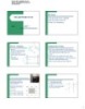
Rendering Pipeline: 3-D Các giải thuật sinh các thực thể cơ sở Transform Illuminate Transform Clip Project Le Tan Hung hunglt@it-hut.edu.vn Rasterize 0913030731 Model & Camera Rendering Pipeline Framebuffer Display Parameters The Rendering Pipeline: 3-D Phép biến đổi Transformations Scene graph Object geometry z screen space- không gian màn hình z model space Không gian mô hình Modeling Transforms • Các điểm của hệ thống tọa độ 3D thế giới thực (a.k.a. object space or world space) Lighting • Các điểm bóng theo mô hình chiếu sáng z 3 loại phép biến đổi: Calculations – Modeling transforms Viewing Viewing transforms • Các điểm trong mô hình hệ tọa độ Camera hay tọa độ điểm nhìn – Transform – Projection transforms Clipping • Các tọa độ điểm của vùng hình chóp cụt với điểm nhìn xác định Projection • Điểm 2- 2-D theo tọa độ màn hình sau phép chiếu được xén tỉa Transform Rendering: Transformations Rendering: Transformations z Modeling transforms z Viewing transform – Size, place, scale, and rotate objects parts of the – Rotate & translate the world to lie directly in front of model w.r.t. each other the camera – Object coordinates Æ world coordinates z Typically place camera at origin z Typically looking down -Z axis – World coordinates Æ view coordinates Y Y Z X X Z 1
Rendering: Transformations Rendering: Transformations z Projection transform z All these transformations involve shifting – Apply perspective foreshortening z Distant = small: the pinhole camera model coordinate systems (i.e., basis sets) – View coordinates Æ screen coordinates z Oh yeah, that’s what matrices do… z Represent coordinates as vectors, transforms as matrices ⎡X ′⎤ ⎡cos θ −sin θ ⎤ ⎡X ⎤ ⎢ ′⎥ = ⎢ θ ⎥⎢ ⎥ ⎣Y ⎦ ⎣sin cos θ ⎦ ⎣Y ⎦ z Multiply matrices = concatenate transforms! Rendering: Transformations The Rendering Pipeline: 3-D Scene graph z Homogeneous coordinates: represent Object geometry Result: coordinates in 3 dimensions with a 4-vector Modeling Transforms • All vertices of scene in shared 3- 3-D “world” coordinate system – Denoted [x, y, z, w]T z Note that w = 1 in model coordinates Lighting • Vertices shaded according to lighting model Calculations – To get 3-D coordinates, divide by w: [x’, y’, z’]T = [x/w, y/w, z/w]T Viewing • Scene vertices in 3- 3-D “view” or “camera” coordinate system Transform z Transformations are 4x4 matrices Clipping • Exactly those vertices & portions of polygons in view frustum z Why? To handle translation and projection Projection • 2-D screen coordinates of clipped vertices Transform Rendering: Ánh sáng - Lighting The Rendering Pipeline: 3-D Scene graph z Illuminating a scene: coloring pixels according to Object geometry Result: some approximation of lighting Modeling – Global illumination: solves for lighting of the whole Transforms • All vertices of scene in shared 3- 3-D “world” coordinate scene at once system Lighting – Local illumination: local approximation, typically Calculations • Vertices shaded according to lighting model lighting each polygon separately Viewing • Scene vertices in 3- 3-D “view” or “camera” coordinate z Interactive graphics (e.g., hardware) does only Transform system local illumination at run time Clipping • Exactly those vertices & portions of polygons in view frustum Projection Transform • 2-D screen coordinates of clipped vertices 2
Rendering: Clipping Rendering: Xén tỉa - Clipping z Clipping a 3-D primitive returns its intersection z Clipping is tricky! with the view frustum: – We will have a whole assignment on clipping In: 3 vertices Clip Out: 6 vertices Clip In: 1 polygon Out: 2 polygons The Rendering Pipeline: 3-D Modeling: The Basics Transform z Common interactive 3-D primitives: points, Illuminate lines, polygons (i.e., triangles) Transform z Organized into objects Clip – Collection of primitives, other objects Project – Associated matrix for transformations Rasterize z Instancing: using same geometry for multiple objects Model & Camera – 4 wheels on a car, 2 arms on a robot Rendering Pipeline Framebuffer Display Parameters Modeling: The Scene Graph Modeling: The Scene Graph z Đồ thị cảnh scene graph : cây đồ thị lưu trữ đối z Traverse the scene graph in depth-first order, tượng, quan hệ giũa các đối tượng và các phép concatenating transformations biến đổi trên đối tượng đó z Maintain a matrix stack of transformations z Nút là đối tượng; Robot z Cành là các thực thể biến đổi Visited – Tương ứng là các ma trận Robot Head Body Unvisited Mouth Eye Leg Trunk Arm Head Body Matrix Active Stack Foot Mouth Eye Leg Trunk Arm 3
Modeling: The Camera Modeling: The Camera z Finally: need a model of the virtual camera z Camera parameters (FOV, etc) are encapsulated – Can be very sophisticated in a projection matrix z Field of view, depth of field, distortion, chromatic aberration… – Homogeneous coordinates Æ 4x4 matrix! – Interactive graphics (OpenGL): – See OpenGL Appendix F for the matrix z Camera pose: position & orientation – Captured in viewing transform (i.e., modelview matrix) z The projection matrix premultiplies the viewing z Pinhole camera model matrix, which premultiplies the modeling matrices – Field of view – Actually, OpenGL lumps viewing and modeling – Aspect ratio transforms into modelview matrix – Near & far clipping planes Rời rạc hoá điểm ảnh Biểu diễn đoạn thẳng (Scan Conversion rasterization) z Là tiến trình sinh các đối tượng hình học cơ sở bằng z Biểu diễn tường minh phương pháp xấp xỉ dựa trên lưới phân giải của màn (y-y1)/( x-x1) = ( y2-y1)/( x2-x1)1 hình y = kx + m – k = (y2-y1)/( x2-x1) z Tính chất các đối tượng cần đảm bảo : – m = y1- kx1 Δy = k Δx – smooth – P(x2 , y2) – continuous z Biểu diễn không tường minh (y2-y1)x - (x2-x1)y + x2y1 - x1y2 = 0 – pass through specified points hay rx + sy + t = 0 – uniform brightness – s = -(x2-x1 ) u – r = (y2-y1) và t = x2y1 - x1y2 – efficient z Biểu diễn tham biến P(x1, y1) P(u) = P1 + u(P2 - P1) u [0,1] X = x1 + u( x2 - x1 ) Y = y1 + u( y2 - y1 ) m Sinh đường tròn Thuật toán DDA Scan Converting Circles (Digital Differential Analizer) z Explicit: y = f(x) Giải thuật thông thường y = ± R2 − x2 DrawLine(int x1,int y1, int x2,int y2, Thuậttoán ddaline (x1, y1, x2, y2) int color) Usually, we draw a quarter circle by { x1, y1, x2, y2 : tọa độ 2 điểm đầu cuối incrementing x from 0 to R in unit steps float y; k : hệ số góc and solving for +y for each step. int x; x,y,m :biến z Parametric: for (x=x1; x
Giải thuật Bresenham Giải thuật Bresenham z 1960 Bresenham thuộc d2 = y - yi = k(xi +1) + b - yi IBM d1 = yi+1 - y = yi + 1 - k(xi + 1) - z điểm gần với đường thẳng 2 d2 b dựa trên độ phân giai hưu d1 hạn 1 yi+1 d1 z loại bỏ được các phép toán d2z If d1 ≤ d2 => yi+1 = yi + 1 chia và phép toán làm tròn 0 yi như ta đã thấy trong gỉai else d1 > d2 => yi+1 = yi thuật DDA 0 1 2 z D = d1 - d2 z Xét đoạn thẳng với 0 < k < 1 = -2k(xi + 1) + 2yi - 2b + 1 xi xi+1 z Pi = ΔxD = Δx (d1 - d2) Giải thuật Bresenham Giải thuật trung điểm-Midpoint z Jack Bresenham 1965 / Pitteway 1967 Pi = -2Δyxi + 2Δxyi + c Pi+1 - Pi z VanAken áp dụng cho việc sinh các đường thẳng và đường tròn 1985 = -2Δy(xi+1 - xi) + 2Δx(yi+1 - yi) z Các công thức đơn giản hơn, tạo được các điểm tương tự như với Bresenham Ayi+1 z Nếu Pi ≤ 0 ⇒ yi+1 = yi + 1 z d = F (xi + 1, yi + 1/2) là trung điểm của đoạn M Pi+1 = Pi - 2Δy + 2Δx M B AB z Nếu Pi > 0 ⇒ yi+1 = yi ( xi , yi ) Pi+1 = Pi - 2Δy z Việc so sánh, hay kiểm tra M sẽ được thay bằng việc xét giá trị d. xi xi+1 – Nếu d > 0 điểm B được chọn, yi+1 = yi P1 = Δx(d1 - d2) P1 = -2Δy + Δx – nếu d < 0 điểm A được chọn. ⇒ yi+1 = yi + 1 – Trong trường hợp d = 0 chúng ta có thể chọn điểm bất kỳ hoặc A, hoặc B. Bresenham’s Algorithm: Midpoint Bresenham’s Algorithm: Midpoint Algorithm Algorithm z Sử dụng phương pháp biểu diễn không tường minh z If di > 0 then chọn điểm A ⇒ trung điểm tiếp theo sẽ có dạng: ax + by + c = 0 ⎛ 3⎞ ⎛ 3⎞ axi + byi + c = 0 ⇒ ( xi , yi ) on line ⎜ xi + 2, yi + ⎟ ⇒ di+1 = a( xi + 2) + b⎜ yi + ⎟ + c ⎝ 2⎠ ⎝ 2⎠ axi + byi + c < 0 ⇒ ( xi , yi ) above line = di + a + b axi + byi + c > 0 ⇒ ( xi , yi ) below line z Tại mỗi trung điểm của đoạn thẳng giá trị được tính là: ⎛ 1⎞ di = a( xi +1) + b⎜ yi + ⎟ + c ⎝ 2⎠ z Chúng ta gọi di là biến quyết định của bước thứ i 5
Bresenham’s Algorithm: Midpoint Algorithm Midpoint Line Algorithm z if di < 0 then chọn điểm B và trung điểm mới là dx = x_end-x_start dy = y_end-y_start ⎛ 1⎞ ⎛ 1⎞ ⎜ xi + 2, yi + ⎟ ⇒ di+1 = a(xi + 2) + b⎜ yi + ⎟ + c d = 2*dy-dx initialisation z Ta có: ⎝ 2⎠ ⎝ 2⎠ x = x_start = di + a y = y_start a = Δy = yend − ystart ⎫ while x < x_end ⎪ Δy if d
Midpoint Circle Algorithm Midpoint Circle Algorithm z If we assume that the radius is an integral value, then the first d = 1-r x = 0 initialisation pixel drawn is (0, r) and the initial value for the decision variable is given by: y = r stop at diagonal ⇒ end of octant ⎛ 1⎞ ⎛ 2 1⎞ 2 while y < x ⎜1, r − ⎟ ⇒ d0 = 1 + ⎜ r − r + ⎟ − r if d < 0 then ⎝ 2⎠ ⎝ 4⎠ d = d+2*x+3 choose A 5 x = x+1 = −r else 4 d = d+2*(x-y)+5 z Although the initial value is fractional, we note that all other x = x+1 choose B values are integers. y = y-1 ⇒ we can round down: d0 =1 − r endif SetPixel(cx+x,cy+y) endwhile Translate to the circle center Scan Converting Ellipses Scan Converting Ellipses: Algorithm A M tiep tuyen = -1 F ( x, y ) = b 2 x 2 + a 2 y 2 − a 2 b 2 = 0 B gradient B C M z 2a is the length of the major axis along the x axis. z Firstly we divide the quadrant into two regions i z 2b is the length of the minor axis along the y axis. z Boundary between the two regions is z The midpoint can also be applied to ellipses. – the point at which the curve has a slope of -1 – the point at which the gradient vector has the i and j components of z For simplicity, we draw only the arc of the ellipse that equal magnitude lies in the first quadrant, the other three quadrants can be drawn by symmetry grad F(x, y) = ∂F / ∂x i +∂F / ∂y j = 2b2 x i + 2a2 y j Ellipses: Algorithm (cont.) Ký tự Bitmap z At the next midpoint, if a2(yp-0.5)2 z Trên cơ sỏ định nghĩa mỗi ký tự z In region 1, choices are E and SE với một font chư cho trước là một – Initial condition: dinit = b2+a2(-b+0.25) bitmap chữ nhật nhỏ – For a move to E, dnew = dold+DeltaE with DeltaE = b2(2xp+3) z Font/typeface: set of character – For a move to SE, dnew = dold+DeltaSE with shapes DeltaSE = b2(2xp+3)+a2(-2yp+2) z fontcache z In region 2, choices are S and SE – các ký tự theo chuỗi liên tiếp nhau Initial condition: dinit = b2(x trong bộ nhớ p+0.5) +a ((y-1) -b ) – 2 2 2 2 – For a move to S, dnew = dold+Deltas with Deltas = a2(-2yp+3) z Dạng cơ bản ab – For a move to SE, dnew = dold+DeltaSE with – (thường N, nghiêng I, đậm B, DeltaSE = b2(2xp+2)+a2(-2yp+3) nghiêng đậm B+I) z Stop in region 2 when the y value is zero. z Thuộc tính – Also colour, size, spacing and orientation 7
Cấu trúc font chữ Ký tự vector Typedef struct z Xây dựng theo phương { int leftx, pháp định nghĩa các ký tự int width; bởi đường cong mềm bao } Char location; //Vị trí của text ngoài của chúng. Typedef struct z Tốn kém nhất về mặt tính { toán CacheId; Heiglit; // Độ rộng chữ z Chất lượngcao CharSpace; // Khoảng cách giữa các ký tự Charlocation Table [128]; } fontcache Giải thuật đường quét sinh đa giác So sánh Polygon Scan Conversion z Phức tạp (Tính toán z Đơn giản trông việc sinh ký phương trình) z Tồn tại rất nhiều giải thuật sinh đa giác. tự ( copypixel) z Lưu trữ gọn nhẹ z Mỗi giải thuật phục vụ cho 1 loại đa giác nhất z Lưu trữ lớn z Các phép biến đổi dựa vào định: z Các phép biến đổi (I,B, các công thức biến đổi – some algorithms allow triangular polygons only scale) đòi hỏi lưu trữ thêm z Kích thước phụ thuôc vào – others require that the polygons are convex and non self- môi trường ( ko có kích intersecting and have no holes z Kích thước không dổi thước cố định) triangular convex non-convex self-intersecting religious Polygon Scan Conversion Polygon Scan Conversion z Polygon scan conversion là giải thuật chung kinh điển cho các z Dùng giải thuật (trung điểm) để xác loại khác nhau định các điểm biên cho mỗi đa giác z Cho mỗi đoạn thẳng quét, chúng ta xác định các cạnh của đa theo thứ tự tăng của x. giác cắt đoạn thẳng compute spans representing the interior z Các diểm phải: portions of the polygons along this scan-line and fill the – Không bị chia sẻ bởi các đa giác associated pixels. lân cận z This represents the heart of a scan-line rendering algorithm – Các đa giác chỉ toàn các điểm used in many commercial products including Renderman and cạnh( điểm biên) 3D Studio MAX. z Đảm bảo các đa giác chia sẻ điểm biên mà không chia sẻ các điểm ảnh bên trong của mình. 8
Polygon Scan Conversion Polygon Scan Conversion integer x value is on right = exterior z Thủ tục chung: – Xác định giao của đường thẳng quét với cạnh đa giác – Sắp xếp các giao điểm theo mức độ tăng dần của x value – Điền các điểm ảnh vào giữa cặp các điểm x z Need to handle 4 cases to prevent pixel sharing: – if intersection has fractional x value, do we round up or down? z if inside (on left of span) round up, if outside (on right) round down – what happens if intersection is at an integer x value? z if on left of span assume its interior otherwise exterior – how do we handle shared vertices? z ignore pixel associated with ymax of an edge – how do we handle horizontal edges? z handled as a result of previous rule (lower edges not drawn) ymax not horizontal edge removed rounded down for A included rounded up for B Polygon Scan Conversion z Determining intersections with polygon edges is expensive – rather than re-computing all intersections at each iteration, use incremental calculations – i.e. if we intersect edge e on scan-line i then it is likely we will intersect the edge on scan-line i+1 (this is known as edge- coherence) z Assume slope of the edge > 1 (other edges obtained via symmetries) 1 – incremental DDA calculation was: yi +1 = yi + 1, xi+1 = xi + m – slope m is given by m= ( yend − ystart ) (xend − xstart ) – note that numerator and denominator are integral ⇒ we can use integer DDA. 9