


Báo cáo hóa học: "Review Article Techniques to Obtain Good Resolution and Concentrated Time-Frequency Distributions: A Review"
lượt xem 7
download
 Download
Vui lòng tải xuống để xem tài liệu đầy đủ
Download
Vui lòng tải xuống để xem tài liệu đầy đủ
Tuyển tập báo cáo các nghiên cứu khoa học quốc tế ngành hóa học dành cho các bạn yêu hóa học tham khảo đề tài: Review Article Techniques to Obtain Good Resolution and Concentrated Time-Frequency Distributions: A Review
Bình luận(0) Đăng nhập để gửi bình luận!
Nội dung Text: Báo cáo hóa học: "Review Article Techniques to Obtain Good Resolution and Concentrated Time-Frequency Distributions: A Review"
- Hindawi Publishing Corporation EURASIP Journal on Advances in Signal Processing Volume 2009, Article ID 673539, 43 pages doi:10.1155/2009/673539 Review Article Techniques to Obtain Good Resolution and Concentrated Time-Frequency Distributions: A Review Imran Shafi,1, 2 Jamil Ahmad,1, 2 Syed Ismail Shah,1, 2 and F. M. Kashif1, 2, 3 1 Centrefor Advanced Studies in Engineering (CASE), G-5/2 Islamabad, Pakistan 2 IqraUniversity, H-9 Islamabad, Pakistan 3 Laboratory for Electromagnetic and Electronic Systems (LEES), MIT, Cambridge, MA 02139, USA Correspondence should be addressed to Imran Shafi, imran.shafi@gmail.com Received 12 July 2008; Revised 13 December 2008; Accepted 23 April 2009 Recommended by Ulrich Heute We present a review of the diversity of concepts and motivations for improving the concentration and resolution of time- frequency distributions (TFDs) along the individual components of the multi-component signals. The central idea has been to obtain a distribution that represents the signal’s energy concentration simultaneously in time and frequency without blur and crosscomponents so that closely spaced components can be easily distinguished. The objective is the precise description of spectral content of a signal with respect to time, so that first, necessary mathematical and physical principles may be developed, and second, accurate understanding of a time-varying spectrum may become possible. The fundamentals in this area of research have been found developing steadily, with significant advances in the recent past. Copyright © 2009 Imran Shafi et al. This is an open access article distributed under the Creative Commons Attribution License, which permits unrestricted use, distribution, and reproduction in any medium, provided the original work is properly cited. 1. Introduction and Historical Perspective The introduction of time-frequency (t-f) signal process- ing has led to represent and characterize the STSC’ time- varying contents using TFDs [7, 8]. The TFDs are two- The signals with time-dependant spectral content (STSC) dimensional (2D) functions which provide simultaneously, are commonly found in nature or are self-generated for the temporal and spectral information and thus are used many reasons. The processing of such signals forms the to analyze the STSC. By distributing the signal energy basis of many applications including analysis, synthesis, over the t-f plane, the TFDs provide the analyst with filtering, characterization or modeling, suppression, can- information unavailable from the STSC’ time or frequency cellation, equalization, modulation, detection, estimation, domain representation alone. This includes the number of coding, and synchronization [1]. For a practical application, components present in the signal, the time durations, and the STSC can be processed in various ways, other than frequency bands over which these components are defined, time-domain, to extract useful information. A classical tool is the Fourier transform (FT) which offers perfect the components’ relative amplitudes, phase information, and the IF laws that components follow in the t-f plane. There spectral resolution of a signal. However FT possesses intrinsic has been a great surge of activity in the past few years limitations that depend on the signal to be processed. The in t-f signal processing domain. The pioneering work is instantaneous frequency (IF) [2, 3], generally defined as the first conditional moment in frequency ω t , is a useful performed by Claasen and Mecklenbrauker [9–11], Janse and Kaizer [12], and Bouachache [13]. They provided the initial concept for describing the changing spectral structure of the impetus, demonstrated useful methods for implementation, STSC. A signal processing engineer is mostly confronted with and developed ideas uniquely suited to the t-f situation. Also, the task of processing frequencies of spectral peaks which they innovatively and efficiently made use of the similarities require unambiguous and accurate information about the and differences of signal processing fundamentals with IFs present in the signals. This has made the IF a parameter quantum mechanics. Claasen and Mecklenbrauker devised of practical importance in situations such as seismic, radar, many new ideas, procedures and developed a comprehensive sonar, communications, and biomedical application [2–6].
- 2 EURASIP Journal on Advances in Signal Processing where s(t ) is the signal, the distribution is said to be bilinear approach for the study of joint distribtutions [9–11]. How- ever Bouachache [13] is believed to be the first researcher, in the signal because the signal enters twice in its calculation. who utilized various distributions for real-world problems. It possesses a high resolution in the t-f plane, and satisfies a He developed a number of new methods and particularly large number of desirable theoretical properties [1, 28]. It can realized that a distribution may not behave properly in all be argued that more concentration than in the WD would respects or interpretations, but it could still be used if a be undesirable in the sense that it would not preserve the t-f particular property such as IF is well described. Flandrin and marginals. Escudie [14] and coworkers transcribed directly some of the It is found that the spectrogram results in a blurred early quantum mechanical results, particularly the work on version [1, 3], which can be reduced to some degree by the general class of distributions [15, 16] into signal analysis the use of an adaptive window or by the combination of language. The work by Janse and Kaizer [12] developed spectrograms. On the other hand, the use of WD in practical innovative theoretical and practical techniques for the use applications is limited by the presence of nonnegligible of TFDs and introduced new methodologies remarkable in CTs, resulting from interactions between signal components. their scope. These CTs may lead to an erroneous visual interpretation Historically the spectrogram [17–23] has been the most of the signal’s t-f structure, and are also a hindrance to widely used tool for the analysis of time-varying spectra pattern recognition, since they may overlap with the searched and is currently the standard method for the study of t-f pattern. Moreover, if the IF variations are nonlinear, nonstationary signals, which is expressed mathematically as then the WD cannot produce the ideal concentration. Such impediments, pose difficulties in the STSC’ correct analysis, the magnitude-square of the short-time Fourier transform (STFT) of the signal, given by are dealt in various ways and historically many techniques are developed to remove them partially or completely. They 2 were partly addressed by the development of the Choi and x(τ )h(t − τ )e−iωτ dτ , S(t , ω) = (1) Williams distribution [29] in 1989, followed by numerous ideas proposed in literature with an aim to improve the where x(t ) is the signal and h(t ) is a window function TFDs’ concentration and resolution for practical analysis [3, (throughout the paper that follows, we use both i and j for 30–33]. Few other important nonstationary representations √ −1 depending on notational requirements and the limits among the Cohen’s class [1, 15, 34] of bilinear t-f energy for are from −∞ to ∞, unless otherwise specified). The distributions include the Margenau and Hill distribution spectrogram has severe drawbacks, both theoretically, since [35], their smoothed versions [9–11, 36, 37] with reduced it provides biased estimators of the signal IF and group CTs [29, 38–40] are members of this class. Nearly at the delay (GD), and practically, since the Gabor-Heisenberg same time, some authors also proposed other time-varying inequality [24] makes a tradeoff between temporal and signal analysis tools based on a concept of scale rather spectral resolutions unavoidable. However STFT and its than frequency, such as the scalogram [41, 42] (the squared modulus of the wavelet transform), the affine smoothed variation, being simple and easy to manipulate, are still the primary methods for analysis of the STSC and most pseudo-WD (PWD) [43], or the Bertrand distribution commonly used today. [44]. The theoretical properties and the application fields There are alternative approaches [7, 8, 25] with a of this large variety of these existing methods are now motivation to improve upon the important shortcomings well determined, and wide-spread [1, 9–11, 28]. Although of the spectrogram, with an objective to clarify the physical many other QTFDs have been proposed in literature (an and mathematical ideas needed to understand time-varying alphabatical list can be found in [45]), no single QTFD can be effectively used in all possible applications. This is because spectrum. These techniques generally aim at devising a joint different QTFDs suffer from one or more problems. function of time and frequency, a distribution that will be highly concentrated along the IFs present in a signal Nevertheless, a critical point of these methods is their and cross-terms (CTs) free thus exhibiting good resolution. readability, which means both a good concentration of the One form of TFD can be formulated by the multiplicative signal components and no misleading interference terms. comparison of a signal with itself, expanded in different This characteristic is necessary for an easy visual interpre- directions about each point in time. Such formulations tation of their outcomes and a good discrimination between are known as quadratic TFDs (QTFDs) because the repre- known patterns for nonstationary signal classification tasks. sentation is quadratic in the signal. This formulation was An ideal TFD function roughly requires the following four first described by Wigner in quantum mechanics [26] and properties. introduced in signal analysis by Ville [27] to form what (1) High clarity which makes it easier to be analyzed. is now known as the Wigner-Ville distribution (WD). The This require high concentration and good resolution WD is the prototype of distributions that are qualitatively along the individual components for the multicom- different from the spectrogram, and produces the ideal ponent signals. Consequently the resultant TFDs are energy concentration along the IF for linear frequency deblurred. modulated (FM) signals, given by (2) CTs’ elimination which avoids confusion between 1 1 1 noise and real components in a TFD for nonlinear t-f ∗ t − τ s t + τ e−iτω dτ , W (t , ω) s (2) 2π 2 2 structures and multicomponent signals.
- EURASIP Journal on Advances in Signal Processing 3 Table 1: Synthesis of main problems related to QTFDs. Gabor transform Synthesis of major concerns WD Gabor-Wigner transform Worst Clarity Best Reasonably Good Present for multicomponent signals Nil CTs Almost eliminated and nonlinear t-f structures Unsatisfactory Mathematical properties Satisfactory Good Quite Low Computational complexity High Higher (3) Good mathematical properties which benefit to its presented in a sequence developing the ideas and techniques in a logical sequence rather than historical. The effort is on application. This requires that TFDs to satisfy total energy constraint, marginal characteristics and pos- making sections individually readable. itivity issue, and so forth. Positive distributions are everywhere nonnegative, and yield the correct uni- 2. Time-Frequency Analysis variate marginal distributions in time and frequency. A clear distinction between concentration and resolution (4) Lower computational complexity means the time is essential to properly evaluate the TFDs’ performance. needed to represent a signal on a t-f plane. The These concepts have generally been considered synonymous signature discontinuity and weak signal mitigation or equivalent in literature, and terms are often used inter- may increase computation complexity in some cases. changeably. Although one intuitively expects higher concen- A comparison of some popular TFD functions is pre- tration to imply higher resolution, this is not necessarily sented in Table 1. To analyze the signals well, choosing the case [46]. In particular, the CTs in the WD do not an appropriate TFD function is important. Which TFD reduce the auto-component concentration of the WD, which function should be used depends on what application it is considered optimal, but they do reduce the resolution. applies on. On the other hand, the short comings make Although high signal concentration is always desired and is specific TFDs suited only for analyzing STSC with specific often of primary importance, in many applications, signal types of properties and t-f structures. An obvious question resolution may be more important, for example, in the then arise that which distribution is the “best” for a particular analysis of multicomponent dispersive waves and detection situation. Generally there is an attempt to set up a set and estimation of swell [47–49]. There have generally been of desirable conditions and to try to prove that only one two approaches to estimate the time-dependent spectrum of distribution fits them. Typically, however, the list is not nonstationary processes. complete with the obvious requirements, because the author (1) The evolutionay spectrum (ES) approaches [50– knows that the added desirable properties would not be 53], which model the spectrum as a slowly varying satisfied by the distribution he/she is advocating. Also these envelope of a complex sinusoid. lists very often contain requirements that are questionable and are obviously put in to force an issue. As an illustration, (2) The Cohen’s bilinear distributions (BDs) [3], includ- by focusing on the WD and its variants, Jones and Parks [46] ing the spectrogram, which provide a general for- have made an interesting comparative study of the resolution mulation for joint TFDs. Computationally, the ES properties and have shown that the relative performance of methods fall within Cohen’s class. the various distributions depends on the signal. The results There are known limitations and inherent drawbacks show that the pseudo-WD (PWD) is best for the signals with associated with these classical approaches. These pheneom- only one frequency component at any one time, the Choi- ena make their interpretation difficult, consequently, esti- Williams distribution is most attractive for multicomponent mation of the spectra in the t-f domain displaying good signals in which all components have constant frequency resolution has become a research topic of great interest. content, and the matched filter STFT is best for signal components with significant frequency modulation. Jones and Parks have concluded that no TFD can be considered as 2.1. The Methods Based on Evolutionary Spectrum. The ES the best approach for all t-f analysis and both concentration was first proposed by Priestley in 1965. The basic idea is and resolution cannot be improved at one time. to extend the classic Fourier spectral analysis to a more In this paper, we will briefly discuss the basic concepts generalized basis: from sine or cosine to a family of orthog- and well-tested algorithms to obtain highly concentrated and onal functions. In his evolutionay spectral theory, Priestely good resolution TFDs for an interested reader (although represents nonstationary signals using a general class of new ideas are coming up rapidly, we cannot discuss all of oscillatory functions and then defines the spectrum based them due to space limitations). The emphasis will be on on this representation [54]. A special case of the ES used the ideas and methods that have been developed steadily the Wold-Cramer representation of nonstationary processes so that readily understood by the uninitiated. Unresolved [55–58] to obtain a unique definition of the time-dependent issues are highlighted with stress over the fundamentals to spectral density function. According to the Wold-Cramer decomposition, a discrete time nonstationary process x[n] make it interesting for an expert as well. The approaches are
- 4 EURASIP Journal on Advances in Signal Processing can be interpreted as the output of a causal, linear, and time- spectrogram and traditional Gabor expansion [92], provide varying (LTV) system with an impulse response h[n, m], at estimates with poor t-f resolution. time n to an impulse at time m. It is driven by zero-mean The earlier approaches by Akan and Chaparro to obtain stationary white noise e[n] so that high-resolution evolutionary spectral estimates include: averaging estimates obtained using multiple windows [75] n and maximizing energy concentration measure [53]. In [53], x[n] = h[n, m]e[m], the authors proposed a modified Gabor expansion that m=−∞ uses multiple windows, dependent on different scales and (3) n modulated by linear chirps. Computation of the ES with this h[n, m]e−iω(n−m) H ( n, ω ) = expansion provides estimates with good t-f resolution. The m=−∞ difficulties encountered, however, were the choices of scales and in the implementation of the chirping. is the Zadeh’s generalized transfer function (GTF) of the system evaluated on the unit circle. The Wold-Cramer ES of x[n] [56, 57] shows that the The Approach. Akan and Chaparro show that by generalizing time-varying power spectral density of output is equal to and implementing by separating the signal components the magnitude squared of time-varying frequency response using evolutionary masking [75], a much improved spectral of the filter. It is defined as estimate is obtained by an adaptive algorithm [68]. The adaptation uses estimates of the IF of the signal components. 1 2 SES (n, ω) = |H (n, ω)| . The signal is decomposed into its components by means of (4) 2π masking on an initial spectrum of the signal. However, the masking is implemented manually and there is requirement This definition can be viewed as Priestley’s ES provided to perform this action automatically. The estimation of that H (n, ω) is a slowly varying function of n [57]. This the IF of each of the signal component is accomplished restriction removes possible ambiguities in the definition by an averaging procedure. It is shown that using the IF of the spectrum by selecting the slowest of all the possible information of the components in the Gabor expansion time-varying amplitudes for each sinusoid. Without this improves the t-f localization. condition, each signal can have an infinite number of Akan defines a finite-extent, discrete-time signal x(n) as sinusoid/envelope combinations [57]. It has been shown that a combination of linear chirps with time-varying amplitudes the ES and the GTF are related to the spectrogram and as Cohen’s class of BDs [59]. The main objective in deriving and presenting these relations in [59] was to show that the BDs P −1 K −1 and the spectrogram can be considered estimators of the ES. A n, ωk , p ein(ωk +(α p /2)n) , x(n) = (5) A great amount of work is found by Pitton and Loughlin p=0 k=0 to investigate the positive TFDs and their potential appli- cations [60–65]. Pitton and Loughlin utilized the ES and where 0 ≤ n ≤ N − 1, ωk = 2πk/K , and α p is a parameter for Thompson’s multitaper approach [66, 67] to obtain positive selection of scales and slopes for analysis chirps. The selection TFDs, but do not discuss the issue of TFDs’ concentration of scales and slopes for the analysis chirps can be avoided by and resolution. considering a more general model for x(n) than the one given Literature indicates that the pioneering work, remarkable in (5) as [68] in its scope, is performed by Chaparro, Jaroudi, Kayhan, Akan, and Suleesathira. These researchers have not only P −1 K −1 focused on computing the improved evolutionary spectra A n, ωk , p eiφ p (n,k) , x(n) = (6) of nonstationary signals but also innovatively applied the p=0 k=0 concepts to application in various practical situations [50– 53, 68–91]. Their major work includes, signal-adaptive where each of the signal component, x p (n), has a phase evolutionary spectral analysis and a parametric approach for φ p (n, k) to which corresponds an IF ω p (n). Mathematically data-adaptive evolutionary spectral estimation. An interest- the ES of x(n) comes out to be S(n, ωk ) = | p A(n, ωk , p)|2 . ing work is performed by Jachan, Matz, and Hlawatsch on the Akan and Chaparro then implements the evolutionary parametric estimations for underspread nonstationary ran- spectral computation using the multi-window warped Gabor dom processes. The necessary description of these methods expansion [53] for each linear chirp: is presented next. J −1 M −1 K −1 1 a p j , m, k h j (n − mL)einωk , x(n) = 2.1.1. Signal-Adaptive Evolutionary Spectral Analysis. (7) J j =0 m=0 k=0 Although it is well recognized that the spectra of most signals found in practical applications depend on time, here a p refers to Gabor coefficients. The synthesis functions estimation of these spectra displaying good t-f resolution is difficult [3]. The problem lies in the adaptation of the may be obtained by scaling a Gaussian window, g (n), as h j = 2 j/2 g (2 j n), j = 0, 1, . . . , J − 1, where J is the number of scaled analysis methods to the change of frequency in the signal windows, and L < K is the time step in the oversampled components. Constant-bandwidth mehods, such as the
- EURASIP Journal on Advances in Signal Processing 5 6 6 5 5 4 4 Frequency (rad) Frequency (rad) 3 3 2 2 1 1 0 0 50 100 150 200 250 50 100 150 200 250 Time Time (a) (b) Figure 1: Example 1. A signal consisting of two closely spaced quadratic FM components, (a) initial ES estimate of the signal, (b) the final ES estimate (adopted from Akan [68]). Gabor expansion. Necessary simplification of (7) results in with the estimation of the IF of each monocompo- following expression for the evolutionary kernel: nent, ω p (n), and corresponding phase φ p (n, k). This is performed using numeric integration techniques. N −1 x(l)ξ (n, l)e−ilωk , A n, ωk , p = (4) Computation of the final ES, where an estimate of (8) x p (n) in terms of its signal-adaptive Gabor expansion l=0 can be given by where ξ (n, l) is the time-varying window, defined as ξ (n, l) = (1/J ) Jj−1 M=0 γ∗ (l − mL)h j (n − mL) with γ j being an −1 J −1 M −1 K −1 =0 1 j m a p j , m, k h j (n − mL)ei(nωk +φ p (n)) , x p ( n) = analysis window biorthogonal to h j (n) [92]. However (8) J j =0 m=0 k=0 can be viewed as short-time chirp FT with a time-varying (11) window. The adaptive algorithm given by Akan has the following where the Gabor coefficients are calculated according steps. to (1) Computation of an initial ES, S(n, ωk ) = |A(n, ωk )|2 N −1 in (7) and (8) by avoiding the selection of scales and x p (n)γ∗ (n − mL)e−i(nωk +φ p (n)) . a p j , m, k = (12) j slopes for the analysis chirps, that is, taking α p = 0. n=0 (2) Spectral masking of the signal [75], using the initial Akan terms the exponential e−iφ p (n) in (12) as demod- ES, to obtain signal components, x p (n). This masking ulating x p (n) along its IF, to obtain a signal that is of the signal is accompished by multiplying its composed of sinusoids and well represented by Gabor evolutionary kernel A(n, ωk ) by a masking function bases. After calculating the Gabor coefficients of each defined using the initial ES. Thus to get a component component, their spectral representations as in (8) x p (n), a mask can be defined as can be obtained. Finally, the estimation of ES of x(n) ⎧ ⎨1, is possible after compensating for the demodulation ( n, k ) ∈ R p , M p ( n, k ) = ⎩ (9) as 0, otherwise, 2 S(n, ωk ) = A n, ωk − ω p (n), p where R p is a region in the initial ES containing a . (13) single component. Consequently, p A(n, ωk )M p (n, k)einωk , x p (n) = (10) Akan shows by examples that using the IF information of the components in the Gabor expansion, the t-f localization k∈R p is improved. The results are displayed in Figures 1 and 2 this masking is however implemented manually and for signals composed of two closely packed quadratic FM should be done automatically. components and a smiling face consisting of a quadratic FM component, two sinusoids at different time periods, and a (3) Once each component and its spectral representa- tion, A(n, ωk , p) is obtained, the authors proceed Gaussian function shifted in frequency.
- 6 EURASIP Journal on Advances in Signal Processing 3 3 2.5 2.5 Frequency (rad) Frequency (rad) 2 2 1.5 1.5 1 1 0.5 0.5 50 100 150 200 250 50 100 150 200 250 Time Time (a) (b) Figure 2: Example 2. A smiling face signal composed of a quadratic FM component, two sinusoids at different time periods, and a Gaussian function shifted in frequency, (a) initial ES estimate of the signal, (b) the final ES estimate (adopted from Akan [68]). 2.1.2. Data-Adaptive Evolutionary Spectral Estimation—A propose a new estimator that uses information about the Parametric Approach. The ES theory is though mathemat- signal components at frequencies other than the frequency of ically well grounded, but has suffered from a shortage of interest. The DASE computes the spectrum at each frequency estimators. The initial work from Kayhan concentrates on while minimizing the interference from components at other evolutionary periodogram (EP) as an estimator on the line frequencies without making any assumptions regarding these of BDs. His latest work, however, follows a parametric components. This estimator reduces to Capon’s maximum approach in deriving the high-quality estimator for the ES likelihood method [98] in the stationary case. The DASE [50, 51]. Parametric approaches to model the nonstationary has better t-f resolution than the EP and thus it possesses signal using rational models with time-varying coefficients many desirable properties analogous to those of Capon’s represented as expansions of orthogonal polynomial have method. In particular, it performs more robustly than been proposed by various investigators, for example, [93, existing methods when the data is noisy. 94]. However, the validity of their view of a nonstationary The DASE’s mathematical derivation alongwith proper- spectrum as a concatenation of “frozen-time” spectra has ties can be found in [51], and we present here the examples to been questioned [57, 95]. demonstrate the performance of the DASE in comparison to In the earlier effort, Kayhan et al. in [50] proposed the other estimators like the EP and BDs. The first example signal evolutionary periodogram (EP) as an estimator of the Wold- is composed of two chirps: one with increasing frequency Cramer ES. The EP is found to possess many desirable and one with decreasing frequency. Both components have properties and reduces to the conventional periodogram a quadratic amplitude. Figure 4(c) shows the DASE using in the stationary case. It is demonstrated by the authors the Fourier expansion functions. Figure 4(b) shows the EP that the EP outperforms the STFT and various BDs in spectrum using the same expansion functions. Figure 4(a) estimating the spectrum of nonstationary signals. The EP shows the BD using exponential kernels. By comparing the estimator can be interpreted as the energy of the output three plots, it is clear that the DASE approach produces the of a time-varying bandpass filter centered around the best spectral estimate. It outperform the EP by displaying no analysis frequency. To derive the EP, the spectrum at each sidelobes, fewer spurious peaks, and a narrower bandwidth. frequency is found, while minimizing the effect of the signal It also outperforms the BD by producing a nonnegative components at other frequencies under the assumption spectrum with no artifacts and sharper peaks. In the second that these components are uncorrelated or white. Although example, the same signal is imbedded in additive Gaussian this assumption is analogous to the one used in deriving white noise. All the parameters from the example above the conventional periodogram [96], Kayhan and others remain unchanged, and the SNR is 24 dB. Figures 4(d)– realized it to be somewhat unrealistic. The mathemati- 4(f) show the BD, the EP, and the DASE spectral estimates, respectively. This example serves to demonstrate the effect cal details and EP’s properties are discussed in detail in [50, 97]. of noise on each of the methods. Again, the DASE spectrum is found to be the least affected. The EP and the BD Data-Adaptive Evolutionary Spectral Estimator (DASE). In spectra display many more spurious peaks than the DASE order to improve performance, Kayhan et al. [51] further spectrum.
- EURASIP Journal on Advances in Signal Processing 7 processes are useful in many applications such as speech 10 and audio, communications, image processing, computer 5 vision, biomedical engineering, and machine monitoring. A 0 parametric second-order description that is parsimonious −5 in that it captures the time-varying second-order statistics −10 by a small number of parameters is hence of particular 0 255 511 interest. Jachan et al. [76] propose the use of frequency n shifts in addition to time shifts (delays) for modeling (a) nonstationary process dynamics in a physically intuitive 255 way. The resulting parametric models are shown to be equivalent to specific types of time-varying autoregressive moving-average (TVARMA) models. They are parsimonious k 127 for nonstationary processes with small high-lag temporal and spectral correlations (underspread processes), which are 0 frequently encountered in applications. Jachan, Matz, and 0 255 511 Hlawatsch also propose efficient order-recursive techniques n for model parameter estimation that outperform existing (b) estimators for TVARMA (TVAR,TVMA) models with respect to accuracy and/or complexity 255 Major Contributions. Jachan et al. [76] consider a spe- k 127 cial class of TVARMA models that they term t-f ARMA (TFARMA) models. Extending time-invariant ARMA mod- els, which capture temporal dynamics and correlations by 0 0 255 511 representing a process as a weighted sum of time-shifted n (delayed) signal components, TFARMA models additionally use frequency shifts to capture a process’ nonstationarity (c) and spectral correlations. The lags of the t-f shifts used in 255 the TFARMA model are assumed to be small. This results in nonstationary processes with small high-lag temporal k 127 and spectral correlations or, equivalently, with a temporal correlation length that is much smaller than the duration over which the time-varying second-order statistics are 0 0 255 511 approximately constant. Such underspread processes [78, 79] n are encountered in many applications. The TFARMA model and its special cases, the TFAR and TFMA models, are shown (d) to be specific types of TVARMA (AR,MA) models. They 255 are attractive because of their parsimony for underspread processes, that is, nonstationary processes with a limited t- k 127 f correlation structure. The underspread assumption results in parsimony which allows an “underspread approximation” that leads to new, 0 computationally efficient parameter estimators for the 0 255 511 n TFARMA, TFAR, and TFMA model parameters. The authors develop two types of TFAR and TFMA estimators based on (e) linear t-f Yule-Walker equations and on a new t-f cepstrum. Figure 3: Time-varying parametric spectral analysis of the sum of Further, it is shown how these estimators can be combined to two bat echolocation signals: (a) time-domain signal; (b) smoothed obtain TFARMA parameter estimators. In particular, TFAR pseudo-Wigner distribution; (c) TFAR spectral estimate; (d) TFMA parameter estimation can be accomplished via underspread spectral estimate; and (e) TFARMA spectral estimate. Logarithmic t-f Yule-Walker equations with Toeplitz/block-Toeplitz struc- gray-scale representations are used in (b)–(e) (all adopted from ture that can be solved efficiently by means of the Wax- Jachan et al. [76]). Kailath algorithm [80]. Simulation results demonstrate that the proposed methods perform better than existing TVAR, TVMA, and TVARMA parameter estimators with respect 2.1.3. Time-Frequency Models and Parametric Estimators to accuracy and/or complexity. For processes that are not for Random Processes. Nonstationary random processes are underspread (called “overspread” [78, 79]), the proposed more difficult to describe than the stationary processes models by Jachan et al. will not be parsimonious and because their statistics depend on time (or space) [77]. those estimators that involve an underspread approximation Parsimonious parametric models for nonstationary random exhibit poor performance.
- 8 EURASIP Journal on Advances in Signal Processing TFARMA models are physically meaningful due to their spectra. The kernel of this transformation provides the definition in terms of delays and frequency (Doppler) shifts. energy density of the signal in t-f with good resolution This delay-Doppler formulation is also convenient since qualities. With this discrete evolutionary transform a clear the nonparametric estimator of the process’ second-order representation for the signal as well as its t-f energy density statistics that is required for all parametric estimators can is obtained. The authors suggest the use of either the Gabor be designed and controlled more easily in the delay-Doppler or the Malvar discrete signal representations to obtain the domain. Furthermore, TFARMA models are formulated in kemel of the transformation. The signal adaptive analysis a discrete-time, discrete-frequency framework that allows is then possible using modulated or chirped bases, and can the use of efficient fast FT algorithms. They can be applied be implemented with either masking or image segmentation in a variety of signal processing tasks, such as time- on the t-f plane. An interesting approach is a piecewise varying spectral estimation (cf. [81]), time-varying predic- linear approximation of the IF, concentrated along the tion (cf. [82–84]), time-varying system approximation [85], individual components of signal, using the Hough transform prewhitening of nonstationary processes, and nonstationary (used in image processing to infer the presence of lines or feature extraction. curves in an image) and the evolutionary spectrum (ES) [71]. The efficiency and practicality of this approach lie in localized processing, linearization of the IF estimate, Simulation Results. Jachan et al. check the accuracy of the recursive correction, and minimum problems due to CTs proposed TFAR, TFMA, and TFARMA parameter estimators in the TFDs or in the matching of parametric models. by applying them to signals synthetically generated accord- This procudere is innovatively used in jammer excision ing to the respective model. Here the application of the techniques, where unambiguous IF for a jammer composed TFAR, TFMA, and TFARMA models is presented for time- of chirps can be estimated, using ES and Hough transform. varying spectral analysis of the quasi-natural signal shown Also Barbarossa in [72] proposed a combination of the in Figure 3(a). The considered signal is the sum of two WD and the Hough transform for detection and parameter echolocation chirp signals emitted by a Daubenton’s bat estimation of chirp signals in a problem of detection of (http://www.londonbats.org.uk). A smoothed pseudo-WD lines in an image, which is the WD of the signal under (SPWD) [86, 87] of this signal is shown in Figure 3(b). analysis. This method provides a bridge between signal The analysis based on TFAR, TFMA, and TFARMA is and image processing techniques, is asymptotically efficient, performed on this signal using the parameter estimators. and offers a good rejection capability of the CTs, but it From the estimated TFAR, TFMA, or TFARMA parame- has an increased computational complexity. Barbarossa et ters, the corresponding parametric spectral estimates are al. further proposed an adaptive method for suppressing computed, that is, estimates of the ES (TFMA case) or of wideband interferences in spread spectrum communications its underspread approximation (TFAR and TFARMA cases, based on high-resolution TFD of the received signal [73]. resp.). The authors estimate the model orders by means of The approach is based on the generalized Wigner-Hough the AIC [88, 89] and stablize all parameters by means of the Transform as an effective way to estimate the clear picture technique described in [88], with an appropriate stabilization of the IF of parametric signals embedded in noise. The parameter. proposed method provides the advantages like, (1) it is able The spectral estimates are depicted in Figures 3(c)– to reliably estimate the interference parameters at lower SNR, 3(e). It is seen that the TFAR spectrum displays the two exploiting the signal model, (2) the despreading filter is chirp components fairly well, although there are some optimal and takes into account the presence of the excision spurious peaks (this effect is well known from AR models filter. The disadvantage of the proposed method, besides the [90]) and the overall resolution is poorer than that of the higher computational cost, is that it is not robust against nonparametric SPWD in Figure 3(b). The TFMA spectrum, mismatching between the observed data and the assumed as expected, is unable to resolve the timevarying spectral model. peaks of the signal. Finally, the TFARMA spectrum exhibits Chaparro and Alshehri [74], innovatively obtain better better resolution than the SPWD, and it does not contain spectral esimates and use it for the jammer excision in direct any CTs as does the SPWD [87]; on the other hand, the t- sequence spread spectrum communications when the jam- f localization of the components deviates slightly from that mers cannot be parametrically characterized. The authors in the SPWD. As indicated, the important point to note is proceed by representing the nonstationary signals using the that these parametric spectra involve only 30 (TFAR and t-f and the frequency-frequency evolutionary transforma- TFARMA) or 42 (TFMA) parameters. tions. One of the methods, based on the frequency-frequency representation of the received signal, uses a deterministic masking approach while the other, based in nonstationary 2.1.4. Miscellaneous Approaches. We find a considerable Wiener filtering, reduces interference in a mean-square amount of work by a number of researchers in achieving fashion. Both of these approaches use the fact that the good resolution ES and applying the results and related spreading sequence is known at the transmitter and the theory to many fields, specially where nonstationary signals receiver, and that as such its evolutionary representation arise. The purpose of their work has ranged from the can be used to estimate the sent bit. The difference in simple graphic presentation of the results to sophisticated performance between these two approaches depends on the manipulations of spectra. The authors in [70] propose a support rather than on the type of jammer being excised. new transformation for discrete signals with time-varying
- EURASIP Journal on Advances in Signal Processing 9 60 60 60 50 50 50 Time (sample) Time (sample) Time (sample) 40 40 40 30 30 30 20 20 20 10 10 10 0 0 0 0.5 1 1.5 2 2.5 0.5 1 1.5 2 2.5 0.5 1 1.5 2 2.5 0 3 0 3 0 3 Frequency (rad) Frequency (rad) Frequency (rad) 1 1 1 0.8 0.8 0.8 Spectrum Spectrum Spectrum 0.6 0.6 0.6 0.4 0.2 0.4 0.4 0 0.2 0.2 60 60 60 −0.2 40 e) e) e) 40 40 0 0 pl pl pl 0 0 0 20 20 20 m m m 1 1 1 (sa (sa (sa 2 2 2 0 3 0 0 Frequency Frequency 3 Frequency 3 e e e (rad (rad (rad m m m ) ) ) Ti Ti Ti (a) (b) (c) 60 60 60 50 50 50 Time (sample) Time (sample) Time (sample) 40 40 40 30 30 30 20 20 20 10 10 10 0 0 0 0.5 1 1.5 2 2.5 0 3 0.5 1 1.5 2 2.5 0.5 1 1.5 2 2.5 0 3 0 3 Frequency (rad) Frequency (rad) Frequency (rad) 1 1 1 0.8 0.8 0.8 Spectrum Spectrum Spectrum 0.6 0.6 0.6 0.4 0.2 0.4 0.4 0 60 0.2 60 0.2 60 −0.2 40 e) e) e) 40 40 0 0 pl pl pl 0 0 0 20 20 20 1 am m m 1 1 (sa (sa 2 s 2 2 0 0 e( 0 3 3 Frequency Frequency Frequency 3 e e (rad (rad (rad m m m ) ) ) Ti Ti Ti (d) (e) (f) Figure 4: Example signals [51]. Signal 1 composed of two chirps, (a) BD using exponential kernels, (b) EP spectral estimate, and (c) DASE spectral estimate. Signal 2 composed of two chirps with additive Guassian white noise (SNR = 24 dB), (d) BD using exponential kernels, (e) EP spectral estimate, and (f) DASE spectral estimate (all adopted from Kayhan et al. [51]). 2 2 2 t t t 0 0 0 −2 −2 −2 −2 −2 −2 0 2 0 2 0 2 ω ω ω (a) (b) (c) Figure 5: TFD of a Gaussian chirp signal: (a) the WD, (b) the LWD, and (c) the SD distribution with L = 8 (adopted from Stankovi´ [108]). c
- 10 EURASIP Journal on Advances in Signal Processing where C (t , ω) is the joint distribution of signal s(t ), and The frequency-frequency masking approach is found to work Ω(θ , τ ) is called the kernel. The term kernel was coined well when the jammer is narrowly concentrated in parts of the frequency-frequency plane, while the Wiener masking by Classen and Mecklenbrauker [9–11]. These two made approach works well in situations when the jammer is spread extensive contributions to general understanding in signal over all frequencies. analysis context along with Janssen [101]. Another term, Shah et al. [99] developed a method for generating which is brought in (14), is the ambiguity function (AF), for which there are a number of minor differences in an informative prior when constructing a positive TFD by the method of minimum cross-entropy (MCE). This prior terminology. We will use the definition given by Rihaczek, results in a more informative MCE-TFD, as quantified via who defines AF as [102] entropy and mutual information measures. The procedure s∗ (t − τ )s(t )eiθt dt , A(t , τ ) = allows any of the BDs to be used in the prior, and the TFDs (15) obtained by this procedure are close to the ones obtained by the deconvolution procedure at reduced computational cost. consequently (14) may be expressed as the FT of product of Shah along with Chaparro [91, 97] considered the use of the ambiguity and kernel functions, given as TFDs for the estimation of GTF of an LTV filter with a goal C (t , ω) = F {A(θ , τ ) · Ω(θ , τ )}, (16) that once it is blurred, it produces the TFD estimate. They used the fact that many of these distributions are written as where A(θ , τ ) is Woodward AF [103], which has been blurred versions of the GTF and made use of deconvolution an important tool in analyzing and constructing signals technique to obtain the deblurred GTF. The technique is associated with radar [102]. By constructing signals having found general and can be based on any TFD with many a particular AF, desired performance characteristics are advantages like (i) it estimates the GTF without the need achieved. A comprehensive discussion of the AF can be for orthonormal expansion used in other estimators of the found in [102], and shorter reviews of its properties and ES, (ii) it does not require the semistationarity assumption applications are found in [104, 105]. Also a number of used in the existing deconvolution techniques, (iii) it can be excellent articles exploring the relationship between AF and used on many TFDs, (iv) the GTF obtained can be used to the TFDs can be found in [11, 106, 107]. reconstruct the signal and to model LTV systems, and (v) the Many divergent attitudes toward the meaning, inter- resulting ES estimate out performs the ES obtained by using pretation and use of Cohen’s BDs have arisen over the the existing estimation techniques and can be made to satisfy years, with extensive research for obtaining good resolution the t-f marginals while maintaining positivity. and high concentration along the individual components. The Power Spectral Density of a signal calculated from The divergent viewpoints and interests have led to a better the second-order statistics can provide valuable information understanding and implementation. The subject is evolving for the characterization of stationary signals. This informa- rapidly and most of the issues are open. However it is tion is only sufficient for Gaussian and linear processes. important to understand the ideas and arguments that have Whereas, most real-life signals, such as biomedical, speech, been given, as variations and insights of them have led way and seismic signals may have non-Gaussian, nonlinear, and to further developments. nonstationary properties. Addressing this issue, Unsal Artan et al. [100] have combined the higher-order statistics and 2.2.1. The Scaled-Variant Distribution—A TFD Concentrated the t-f approaches and present a method for the calculation along the IF. In an important set of papers, Stankovic et of a Time-Dependent Bispectrum based on the positive al. [33, 108–110] innovatively used the similarities and distributed ES. This idea is particularly useful for the analysis differences with quantum mechanics and originated many of such signals and to analyze the time-varying properties of new ideas and procedures to achieve the good resolution and nonstationary signals. high concentration of joint distributions. Their initial work suggests the use of the polynomial WD [30, 111] to improve 2.2. The Methods Based on Cohen’s Bilinear Class. In 1966 the concentration of monocomponent signals, taking the IF as a method was devised that could generate in a simple polynomial function of time. A similar idea for improving manner an infinite number of new ones [3, 15]. The the distribution concentration of the signal whose phase is approach characterizes TFDs by an auxiliary function and polynomial up to the fourth order was presented in [25]. by the kernel function. We will discuss the significant In order to improve distribution concentration for a signal contributions on high spectral resolution kernels later in this with an arbitrary nonlinear IF, the L-Wigner distribution paper. The properties of distribution are reflected by simple (LWD) was proposed and studied in [25, 112–115]. The constraints on the kernel, and by examining the kernel one polynomial WD, as well as the LWD, are closely related to readily can ascertain the properties of the distribution. This the time-varying higher-order spectra [111, 114–116]. They allows one to pick and choose those kernels that produce were found to satisfy only the generalized forms of marginal distributions with prescribed desirable properties. All TFDs and unable to preserve the usual marginal properties [1, 28]. can be obtained from a general expression 1 1 1 s∗ μ − τ s μ + τ Ω(θ , τ ) C (t , ω ) = 2 Variant of LWD. Lately Stankovic proposed a variant of LWD 4π 2 2 (14) obtained by scaling the phase and τ axis by an integer L × e−iθt−iτω+iθμ dμdτdθ , while keeping the signals’ amplitudes unchanged [33, 108].
- EURASIP Journal on Advances in Signal Processing 11 −1 −1 −1 t t t 0 0 0 1 1 1 −64π −64π −64π 64π 64π 64π ω ω ω (a) (b) (c) Figure 6: TFD of a signal with fast amplitude variations: (a) the WD, (b) the LWD with L = 2, and (c) the SD distribution with L = 2 (adopted from Stankovi´ [108]). c with uncertainty of the order of 1/L2 while at the same time He terms this new distribution as the scaled variant of the LWD (SD) of a signal x(t ). It is defined, in its pseudo form, keeping other important properties of the TFD invariant by keeping L slightly greater than 1 (L = 2, 4, . . .). It is shown as through example of Gaussian chirpsignal and a noisy signal τ τ −iωτ ωL (τ )x[L] t + x[L]∗ t − SDL (t , ω) = e dτ. with same order of amplitude and phase variations (see Figures 2L 2L 5 and 6) that the SD produces the ideal concentration at the (17) IF. The word “pseudo” is used to indicate the presence of the window ωL (τ ) where x[L] (t ) is the modification of x(t ) Realization of the SD. A method for the direct realization obtained by multiplying the phase function by L while of the SD, based on the straightforward application of a keeping the amplitude unchanged: distribution definition, is presented in [110]. In the case of multicomponent signals, it may be equal to the sum x[L] (t ) = A(t )eiLφ(t) . (18) of the SDs of each component separately. For the SD in (17), signal x(t ) is modified into xL (t ), oversampled L times, The distribution achieves high concentration at the IF— while the number of samples that are used for calculation as high as the LWD—while at the same time satisfying time is kept unchanged. This method is not computationally marginal and unbiased energy condition for any L. The much more demanding than the realization of any ordinary frequency marginal is satisfied for asymptotic signals as well. (L = 1) distribution. In the case of multicomponent signals, this method produces signal power concentrated Simulation Results. The original idea for this distribution at the resulting IF, according to the theorem presented stems from the very well-known quantum mechanics forms. in [108]. Theory is illustrated on the numerical examples There is a partial formal mathematical correspondence of multicomponent real signal, real noisy multicomponent between quantum mechanics and signal analysis. Relation- signal, and a multicomponent signal whose components ship between quantum mechanics and signal analysis may intersect (see Figures 7 and 8). The proposed distributions be found in [1] and is beyond the scope of this paper. may achieve arbitrary high concentration at the IF, satisfying Historically, work on joint TFDs has often been guided by the marginal properties. Till the publication of [110], this corresponding developments in quantum mechanics. The was possible only in a very special case of the linear frequency similarity comes about because in quantum mechanics the modulated signal using the WD. probability distribution for finding the particle at a certain position is the absolute square of the wave function, and the probability for finding the momentum is the absolute 2.2.2. Reassigned TFDs. Some TFDs were proposed to adapt square of the FT of the wave function. Thus one can associate to the signal t-f changes. In particular, an adaptive TFD can the signal with the wave function, time with position, and be obtained by estimating some pertinent parameters of a signal-dependant function at different time intervals [45]. frequency with momentum. The marginal conditions are formally the same, although the variables are different. Such TFDs provide highly localized representations without suffering QTFDs’ CTs. The tradeoff is that these TFDs Consequently for a signal x(t ) = A(t )eiφ(t) , a function Ψ(λ) = A(λ)eiLφ(λ) can be formed that corresponds (with may not satisfy some desirable properties such as energy L = 1/ D) to the Wentzel solution of the Schroedinger’s preservation. Examples of adaptive TFDs include the high equation or to the Feynman’s path integral [108]. This form resolution TFD [117], the signal-adaptive optimal-kernel applied to the original quantum mechanics form of the WD TFDs [118, 119], the optimal radially Gaussian TFD [120], WD(λ, p) = Ψ(λ + Dτ/ 2)Ψ∗ (λ − Dτ/ 2)e−ipτ dτ produces and Cohen’s nonnegative distribution [34]. Reassigned TFDs the proposed SD exactly. It is shown that significant benefit also adapt to the signal by employing other QTFDs of the with respect to the distribution concentration is possible signal such as the spectrogram, the WD, or the scalogram
- 12 EURASIP Journal on Advances in Signal Processing However x(t ) can be reconstructed from the moving [121–127]. The former types of adaptive TFDs are discussed window coefficients by under the name Optimal-kernel TFDs in Section 2.2.3. The method of reassignment improves considerably the t-f concentration and sharpens a TFD by mapping the data Xτ (ω)h∗ (τ − t )dωdτ x(t ) = ω to t-f coordinates that are nearer to the true region of support of the analyzed signal. The method has been independently Xτ (ω)h(τ − t )e− jω(τ −t) dωdτ = introduced by several researchers under various names [121– 127], including method of reassignment, remapping, t-f (21) reassignment, and modified moving-window method. In Mτ (ω)e jϕτ (ω) h(τ − t )e− jω(τ −t) dωdτ = the case of the spectrogram or the STFT, the method of reassignment sharpens blurry t-f data by relocating the data Mτ (ω)h(τ − t )e j [ϕτ (ω)−ωτ +ωt] dωdτ. = according to local estimates of the IF and GD. This mapping to reassigned t-f coordinates is very precise for signals that are separable in time and frequency with respect to the analysis For signals having magnitude spectra, M (t , ω), whose time window. variation is slow relative to the phase variation, the maxi- mum contribution to the reconstruction integral comes from The Reassignment Method. Pioneering work on the method the vicinity of the point t , ω satisfying the phase stationarity of reassignment was first published by Kodera et al. under condition the name of modified moving window method [124]. Their technique enhances the resolution in time and frequency ∂ ϕτ (ω) − ωτ + ωt = 0, of the classical moving window method (equivalent to the ∂ω (22) spectrogram) by assigning to each data point a new t-f ∂ coordinate that better reflects the distribution of energy ϕτ (ω) − ωτ + ωt = 0, ∂τ in the analyzed signal. This clever modification of the spectrogram unfortunately remained unused because of implementation difficulties and because its efficiency was or equivalently, around the point t , ω defined by not proved theoretically. Later on, Auger and Flandrin [121] ∂ϕτ (ω) ∂ϕτ (τ , ω) showed that this method, which they called the reassignment t (τ , ω) = τ − =− , method, can be applied advantageously to all the bilinear t-f ∂ω ∂ω (23) and time-scale representations, and can be easily computed ∂ϕτ (ω) ∂ϕτ (τ , ω) ω= =ω+ for the most common ones. Independently of Kodera et . ∂τ ∂τ al., Nelson arrived at a similar method for improving the t-f precision of short-time spectral data from partial The t-f coordinates thus computed are equal to the local derivatives of the short-time phase spectrum [125]. It is GD, tg (t , ω), and local IF, ωi (t , ω), and are computed from easily shown that Nelson’s cross-spectral surfaces compute the phase of the STFT, which is normally ignored when an approximation of the derivatives that is equivalent to the constructing the spectrogram. These quantities are local in finite differences method. the sense that they are represent a windowed and filtered In the classical moving window method [128], a time- signal that is localized in time and frequency, and are not domain signal, x(t ), is decomposed into a set of coefficients, global properties of the signal under analysis. ∈ (t , ω), based on a set of elementary signals, hω (t ), defined The modified moving window method, or method of as reassignment, changes (reassigns) the point of attribution of ∈ (t , ω) to this point of maximum contribution tg (t , ω), hω (t ) = h(t )e jωt , (19) ωi (t , ω), rather than to the point t , ω at which it is computed. where h(t ) is a (real-valued) low-pass kernel function, like This point is sometimes called the center of gravity of the the window function in the STFT. The coefficients in this distribution, by way of analogy to a mass distribution. This analogy is a useful reminder that the attribution of decomposition are defined as spectral energy to the center of gravity of its distribution x(τ )h(t − τ )e− jω(τ −t) dτ ∈ (t , ω ) = only makes sense when there is energy to attribute, so the method of reassignment has no meaning at points where the spectrogram is zero valued. x(τ )h(t − τ )e− jωτ dτ = e jωt (20) Efficient Computation of Reassigned Times and Frequencies. = e jωt X (t , ω) The reassignment operations proposed by Kodera et al. cannot be applied directly to the discrete STFT data, because = Xt (t , ω) = Mt (ω)e jϕτ (ω) , partial derivatives cannot be computed directly on data that where Mt (ω) is the magnitude, and ϕτ (ω) is the phase, of is discrete in time and frequency, and it has been suggested that this difficulty has been the primary barrier to wider use Xt (ω), the FT of the signal x(t ) shifted in time by t and windowed by h(t ). of the method of reassignment.
- EURASIP Journal on Advances in Signal Processing 13 ω ω 256π 256π 0 0 0 0 t t 1 1 (a) (b) ω 256π 0 0 0 t t 1 (c) 1 ω |X(w)| 2 256π 0 0 256π 0 ω t (d) 1 (e) ω ω 256π 256π 0 0 0 0 t t 1 1 (f) (g) Figure 7: TFD of a multicomponent signal: (a) the spectrogram, (b) the WD, (c) the S-method, (d) the S-distribution with L = 2, including marginal properties, (e) the S-distribution with L = 2, (f) the S-method of noisy signal, (g) the S-distribution with L = 2 of noisy signal (adopted from Stankovi´ [110]). c dΩ Auger and Flandrin [121] showed that the method of TFD(x; t , ω) = φTF (u, Ω)WD(x; t − u, ω − Ω)du , 2π reassignment, proposed in the context of the spectrogram (24) by Kodera et al., could be extended to any member of Cohen’s class of TFDs by generalizing the reassignment operations. Auger and Flandrin’s starting point of the which shows the 2D low-pass filtering of the WD, leading to efficient reassignment method is a TFD of the Cohen’s class [3, 15]. However, this smoothing
- 14 EURASIP Journal on Advances in Signal Processing ω ω −64π −64π 64π 64π −1 −1 t t 1 1 (a) (b) Figure 8: TFD of a multicomponent signal whose components intersects: (a) spectrogram, (b) S-distribution with L = 2 (adopted from Stankovi´ [110]). c where δ (t ) denotes the Dirac impulse. It should be noticed also produces a less accurate t-f localization of the signal components. Its shape and spread must therefore be properly that the aim of the reassignment method is to improve the determined so as to produce a suitable tradeoff between sharpness of the localization of the signal components by good interference attenuation and good t-f concentration reallocating its energy distribution in the t-f plane. Thus, [1, 28, 29]. Interesting examples of smoothings are the PWD when the representation value is zero at one point, it is useless [9–11], the SPWD [36], and all the reduced interference dis- to reassign it. Equations (25), the reassignment operators, tributions [29, 39, 40]. As a complement to this smoothing, have therefore neither sense nor use in this case. It should be also noticed that if the smoothing kernel φTF (u, Ω) is real other processings can be used to improve the readability of a signal representation. A kind of signal representation valued, the reassignment operators (25) are also real valued, processing, to which the reassignment method belongs, is to since the WD is always real valued. perform an increase of the signal components concentration. The above expression shows that the value of a TFD at Simulation Results. In order to evaluate the benefits of the any point (t , ω) of the t-f plane is the sum of all the terms reassignment method in practical applications, a comparison φTF (u, Ω)WD(x; t − u, ω − Ω), which can be considered as the of the experimental results provided by some TFDs and contributions of the weighted WD values at the neighboring their modified versions is shown in this section, adopted points (t − u, ω − Ω). TFD(x; t , ω) is then the average of from Auger and Flandrin [121]. Auger and Flandrin ana- the signal energy located in a domain centered on (t , ω) lyze a 256-point computer-generated signal made up of and delimited by the essential support of φTF (u, Ω). This one sine wave component, one chirp component, one averaging leads to the attenuation of the oscillating CTs, but chirped Gaussian packet, and one signal with constant also a signal components broadening. The TFD can hence be amplitude and an instantaneous frequency describing half nonzero on a point (t , ω) where the WD indicates no energy, a sine period. Figure 9(a) shows the SPWD, adding a time- if there are some nonzero WD values around. Therefore, one direction smoothing to PWD. There are very few CTs, but the way to avoid this is to change the attribution point of this signal components concentration is still weaker. Its modified average, and to assign it to the center of gravity of these version (shown in Figure 9(b)) is nearly ideal: all CTs are energy contributions, whose coordinates are removed by the smoothings, and the signal components are strongly localized by the reassignment method. If the u · φTF (u, Ω)WD(x; t − u, ω − Ω)du(dΩ/ 2π ) t (x; t , ω)= t − time and frequency smoothing windows are equal, the , φTF (u, Ω)WD(x; t − u, ω − Ω)du(dΩ/ 2π ) representation becomes then the spectrogram (Figure 9(c)), whose modified version (Figure 9(d)) perfectly localizes the Ω · φTF (u, Ω)WD(x; t − u, ω − Ω)du(dΩ/ 2π ) ω(x; t , ω)= ω − , chirp component. Finally, the next figures show time-scale φTF (u, Ω)WD(x; t − u, ω − Ω)du(dΩ/ 2π ) representations. The affine PWD performs a scale-invariant (25) frequency direction smoothing of the WD. Its modified version yields much more concentrated signal components, rather than to the point (t , ω) where it is computed. This but still retains some CTs. An additional scale-invariant reassignment leads to the construction of a modified version time direction smoothing removes nearly all CTs, yielding of this TFD, whose value at any point (t , ω ) is therefore the an affine SPWD (Figure 9(e)) with less concentrated signal sum of all the representation values moved to this point: components, and a nearly ideal modified affine SPWD (Figure 9(f)). Figure 9(g) now shows a scalogram whose MTFD(x; t , ω ) = TFD(x; t , ω)δ t − t (x; t , ω) window length was chosen to provide the same frequency direction smoothing, but (consequently) an approximately (26) dω two times longer time direction smoothing than the previous × δ (ω − ω(x; t , ω))dt , affine SPWD. All the WD CTs have been removed, but 2π
- EURASIP Journal on Advances in Signal Processing 15 ×10 ×10 25.6 25.6 19.2 19.2 12.8 12.8 6.4 6.4 0 0 6.4 12.8 19.2 25.6 6.4 12.8 19.2 25.6 0 0 ×10 ×10 (a) (b) ×10 ×10 25.6 25.6 19.2 19.2 12.8 12.8 6.4 6.4 0 0 6.4 12.8 19.2 25.6 6.4 12.8 19.2 25.6 0 0 ×10 ×10 (c) (d) ×10 ×10 25.6 25.6 19.2 19.2 12.8 12.8 6.4 6.4 0 0 6.4 12.8 19.2 25.6 6.4 12.8 19.2 25.6 0 0 ×10 ×10 (e) (f) ×10 ×10 25.6 25.6 19.2 19.2 12.8 12.8 6.4 6.4 0 0 6.4 12.8 19.2 25.6 6.4 12.8 19.2 25.6 0 0 ×10 ×10 (g) (h) Figure 9: Numerical examples for reassignment method for a 4-component signal made up of a sine wave component, a chirp component, a chirped Gaussian packet, and one signal with constant amplitude and an IF describing half a sine period, (a) SPWD. h : 79-point Gaussian window, (b) modified version of the SPWD, (c) spectrogram. h : 31-point Gaussian window, (d) modified version of the spectrogram, (e) affine SPWD. h: Gaussian window with F0 · Th = 4.24, (f) modified version of affine SPWD, (f) scalogram. h: Gaussian window with F0 · Th = 3.0, (h) modified version of the scalogram (all adopted from Auger and Flandrin [121]). the time resolution is really inadequate, especially at low 2.2.3. Optimal-Kernel TFDs. The result in (14) to (16) frequencies. Its modified version is much easier to interpret, indicate that a quadratic TFD is obtained by first smoothing but the localization of the component with sinusoidal the symmetric AF (using the kernel function) and then by frequency modulationcy seems weaker than on the affine taking a 2D FT of the result. This result is equivalent to SPWD. a 2D filtering in the ambiguity domain. The properties of
- 16 EURASIP Journal on Advances in Signal Processing distribution are reflected by simple constraints on the kernel autocorrelation function via autoregressive (AR) modeling and have been used advantageously to develop practical techniques [131–135]. Such parameterization seeks to fit a methods for analysis and filtering, as was done by Eichmann least-squares random model to the second-order statistics of the LAF at different time instants. The AR modeling and Dong [129]. Excellent reviews relating the properties of the kernel to the properties of the distribution have techniques, however, view the LAF as a stationary process been given by Janse and Kaizer [12], Janssen [101], Claasen along the lag dimension. Since t-f distribution kernels and Meclenbrauker [11], and Boashash [7]. By examining translate deterministic signals into others of deterministic the kernel one readily can ascertain the properties of the nature, it will be more appropriate to fit a deterministic, distribution. This allows one to pick and choose those rather than a stochastic, model to the LAF. Further, all kernels that produce distributions with prescribed desirable modeling techniques applied in the TFD context mostly have properties. Thus, by a proper choice of kernel function, only dealt with PWD or the SPWD kernels. one can reduce or remove the CTs in the analysis of Amin and Williams [130] have maintained that in addi- multicomponent signal. This unified approach is simple with tion to PWD and SPWD of separable time and lag windows, an advantage that all distributions can be studied together in there exists a large class of t-f kernels for which the LAF a consistent way. Since for any given signal some TFDs are is amenable to high spectral resolution techniques. The “better than others,” kernel design has become an important members of this class satisfy the desirable t-f properties for research area. Generally the optimum kernel TFDs can be achieved by three different approaches to optimizing the power localization in nonstationary environment, yet they produce local autocorrelation functions that are amenable kernel with an aim to improve the resolution of resulting TFDs, which are to exponential deterministic modeling during periods of stationarity. The proposed high spectral resolution ker- (1) high resolution TFDs based on high spectral resolu- nels are, however, required to meet two basic conditions tion kernels; [130]: (2) high resolution TFDs based on signal-independant (1) the frequency marginal, kernels; (2) an exponential behavior in the ambiguity domain for (3) high resolution TFDs based on signal-dependant constant values of few parameters. kernels; In dealing with sinusoidal data, the first property guarantees that the autoterm sinusoids in the LAF are High Resolution TFDs-High Spectral Resolution Kernels. undamped. The second property enforces an exponential TFDs along with their temporal and spectral resolutions damping on all CTs. As a result, the sinusoidal components are uniquely defined by the employed t-f kernels. Potential in the data translate into damped/undamped sinusoids in the kernels seek to map, at every time sample, the time- local autocorrelation function. High-resolution techniques varying signals in the data into approximately fixed fre- such as reduced rank approximation of the backward linear quency sinusoids in the local autocorrelation function (LAF). prediction data matrix can then be applied for frequency esti- Applying the FT to the LAF, therefore, provides a peaky mation. The authors use Prony’s method and its least squares spectrum where the location of the peaks is indicative reduced-order approximation based on the singular value to the signals’ instantaneous power concentrations. The decomposition (SVD) [136, 137] in the t-f context. This sinusoidal components in the LAF, however, generally method is shown to be applicable to high spectral resolution appear with some type of amplitude modulations (AMs), TFD problems, specifically when the underlying LAF is made which are highly dependent on the kernel composition up of a sum of exponentially damped/undamped sinusoids [130]. Such modulation presents a limitation on spectral or chirp-like signals. The authors derive a class of TFD resolution in the t-f plane, as it is likely to spread both kernels in which the autoterms and the CTs of the sinusoidal the auto and CTs to localizations over a wide range of frequencies. components in the data are, respectively, mapped into undamped and damped sinusoids. By using the backward A. Improving TFDs’ Spectral Resolution. Because of the kernel modulation effects on the various terms, closely linear prediction frequency estimation approach [136], these two sets of components produce a linear predictor error filter spaced frequencies may not be resolved. Further, since TFDs whose zeros lie on and outside the unit circle, respectively. are Fourier based, then in addition to the AM imposed by With the extraneous zeros of the polynomial lying inside the kernels, the spectral resolution is limited by and highly the unit circle, fitting a deterministic model to the LAF of dependent on the extent of LAF, that is, the lag window the proposed class of t-f kernels not only yields accurate employed [130]. However, increasing the length of the LAF estimates of the frequencies of the sinusoids but also provides will not always yield improved resolution. Events occurring a mechanism to distinguish between the true and false over short periods of time do not require large kernels, which distribution terms. may only lead to increased CT contributions from distant B. Simulation Results. The simulations in Figures 10 and events and obscure the local autoterms. Limited availability 11 high spectral resolution kernels illustrate the effectiveness of data samples may also provide another reason for using of the high-resolution TFDs achieved by the high spectral small extent kernels. In these cases, improving spectral reso- resolution kernels. A test signal is constructed that consisted lution of a TFD can be achieved by parameterizing its local
- EURASIP Journal on Advances in Signal Processing 17 of two complex exponentials as kernel is given by α |τ | G( t , τ ) = , (28) i2π 12.8(n−30)/ 128 i2π 51.2n/ 128 x(n) = e n = 0, 1, 2, . . . , 127. cosh2 (t ) +e , (27) further it can be written as 2D ambiguity domain filter, given by These two signals’ components have normalized frequencies G(t , τ )e−i2πυt dt , of 0.1 and 0.4 Hz, respectively. First, the authors compute g (υ, τ ) = (29) the binomial TFD using the alias free formulation [39] for comparison. The LAF, which extended to 128 points, where υ and τ are the two usual variables in the ambiguity is computed, and the binomial kernel is applied to it. domain. Using (29) in the general formula of the QTFDs, the Applying an FFT across the lags produced the result shown authors come up with the following discrete-time version of in Figure 10(a). The two components are well resolved, and the proposed TFD on simplification: the CT interference is low. Figure 10(b) shows the high- resolution TFD result using the binomial kernel. Only even M M ρz n, f = G p, m z n + p + m lag terms are used in the LAF. The results are similar to m=−M p=−M the binomial TFD, but the resolution is higher. In addition, (30) the CTs are small and generally fall between the autoterms × z∗ n + p − m e−i2πm f , and are not spread, as is the case for the binomial TFD. Figure 11(a) shows the results obtained using the raw LAF where z(t ) is the analytic multicomponent signal under values, which is equivalent to the PWD. The autoterms are consideration, and the discrete-time expressions G(n, m) and well resolved, but the CTs are as large as in the conventional z(n) are obtained by sampling G(t , τ ) and z(t ) at a frequency PWD and fall between the CTs. A 20-point analysis window fs = 1/T such that t = n · T and τ = m · T . The resulting TFD is used to find the Hankel structure for the odd positive lags in (30) is alias-free and periodic in f with a period equal to obtained from the same LAF used to form the binomial TFD. unity. The authors limit the number of terms included from the Simulation Results. The distribution in (29) is claimed to SVD computation by excluding all terms with magnitudes solve problems that the WD or the spectrogram cannot. In less than 15% of the largest singular value. The effectiveness particular, the proposed distribution is shown to resolve two of the approach with a nonstationary chirp is shown in close signals in the t-f domain that the two other distribu- Figure 11(b). The authors analyze a complex exponential tions cannot. Further synthetic and real data collected from with a starting frequency of 0.05 Hz and a positive chirp rate real-world applications are used to validate the proposed of 0.6 × 10⁻⁴ Hz/sample using the alias-free binomial LAF. distribution (see Figures 12–14). Here, 0.1 Hz spans 100 frequency samples. We can see that the method provides a very nice estimate of the t-f course of Adaptive TFDs—Signal-Dependant Kernel. Adaptive TFDs the signal. are highly localized t-f representations without suffering from CTs, and they can generally be obtained by esti- mating some pertinent parameters of time-varying signal- A High-Resolution QTFD—Signal-Independent Kernel. A dependant function. A great amount of work is performed signal independent kernel for the design of a high-resolution by Baraniuk and Jones, who have developed several different and CTs free quadratic TFD is proposed in [138]. The approaches optimizing the signal-dependant kernel t-f anal- filtering of the CTs in the ambiguity domain that reduces ysis [118–120, 139], including the following: (or removes) the CTs in the t-f domain results in a lower t-f resolution. That is, there is tradeoff between CTs suppression (1) 1/0 optimal kernel TFD [118] formulation in which and t-f resolution in the design of a given quadratic TFD. the optimal kernel turns out to have a special binary Barkat and Boashash propose a kernel that allows retaining structure: it takes on only the values 1 and 0; as many autoterms energy as possible while filtering out as much CTs energy as possible. The kernel is defined in the (2) optimal radially Gaussian kernel TFD [120] temper- time lag domain keeping in view the implementation of the ing the “1/0 kernel” optimization formulation with resultant TFD. an additional smoothness constraint that forces the Beginning from a time function (1/ cosh2 (t )) whose optimal kernel to be Gaussian along radial profiles; spectrum presents the narrowest mainlobe compared with (3) signal adaptive optimal kernal TFDs [119]. many other considered time function for the same signal duration. Barkat and Boashash extend it to a 2D quantity Baraniuk and Jones have made use of the fact that sym- (|τ |/ cosh2 (t )) and then taking it to a power α; they obtain metric AF is the characteristic function of the WD. The two desirable characteristics. First, its FT (kernel function), mathematical and possible physical analogy between the two which is centered around the origin, presents sharp cutoff enhances the interpretation of the properties of the AF. As edges. Second, the volume beneath it can be controlled by an illustration, consider the example of the AF of the bat varying the value of α. Consequently, the proposed time-lag chirp in Figure 15(a). The FT maps the WD autocomponents
- 18 EURASIP Journal on Advances in Signal Processing 1 1 0.8 0.8 0.6 0.6 0.4 0.4 0.2 0.2 0 0 −0.2 −0.4 −0.2 150 100 1 1 100 0.8 0.8 0.6 0.6 Tim 50 Tim 50 0.4 0.4 e sa ency ency e sam mp 0.2 0.2 frequ frequ le ple alised alised 0 0 0 0 Norm Norm (a) (b) Figure 10: TFD results for x(n): (a) bionomial TFD (b) high-resolution bionomial TFD (adopted from Amin and Williams [130]). 0.1 0.09 0.08 2 0.07 1 0.06 Frequency 0.05 0 0.04 −1 0.03 −2 0.02 100 0.01 1 0.8 0.6 50 Tim 0 0.4 ncy e reque sam 0.2 0 20 40 60 80 100 120 ised f ple 0 0 al Norm Sample (a) (b) Figure 11: (a) High-resolution TFD for x(n) using the raw LAF values (PWD equivalent). (b) High-resolution result for a complex exponential signal over 128 time samples (adopted from Amin and Williams [130]). where Φ(θ , τ ) is the kernel function, and the σ (ψ ) is the to a region centered on the origin of the AF plane, whereas it maps the oscillatory WD cross-components away from spread function that controls the spread of the Gaussian at radial angle ψ . The angle ψ ≡ arctan(τ/θ ) is measured the origin. In the AF image 15(a), the AF autocomponents between the radial line through the point (θ , τ ) and the θ corresponding to the three harmonics of the bat chirp lie superimposed at the center of the AF image, while the AF axis. Radially Gaussian kernels can be expressed in polar √ coordinates, using ξ = θ 2 + τ 2 as radius variable: cross-components lie to either side. The components slant in the AF because the bat signal is chirping. The fact that the auto- and cross-components are spatially separated in the ξ2 Φ ξ , ψ = exp − . (32) AF domain facilitates optimization of the kernel function, 2σ 2 ψ which is used as a masking function to the AF to suppress the CTs. The two later concepts based on optimal radially A high-quality TFD results when the kernel is well Gaussian and signal adaptive optimal kernels are discussed matched to the components of a given signal. This technique next to illustrate the work of Baraniuk and Jones. is in contrast to the approach considered by Barkat and A. The Optimal Radially Gaussian TFD. The signal- Boashash [138] described in the last section. This is because dependent TFD proposed in [120] is based on kernels with the radially Gaussian kernel is adapted to a signal by solving Gaussian radial cross section: the following optimization problem: θ2 + τ 2 ∞ 2π Φ(θ , τ ) = exp − 2 , (31) A(ξ , ψ )Φ(ξ , ψ ) ξdξdψ max (33) 2σ 2 ψ Φ 0 0
- EURASIP Journal on Advances in Signal Processing 19 1 1 0.8 Normalised amplitudes Normalised amplitudes 0.6 0.5 0.4 0.2 0 0 −0.2 −0.4 −0.5 0.05 0.1 0.15 0.2 0.25 0.3 0.35 0.4 0.45 0.5 0.05 0.1 0.15 0.2 0.25 0.3 0.35 0.4 0.45 0.5 0 0 Frequency (Hz) Frequency (Hz) Proposed distribution Proposed distribution WVD WVD Spectrogram Spectrogram (a) (b) 1 0.8 Normalised amplitudes 0.6 0.4 0.2 0 −0.2 −0.4 0.05 0.1 0.15 0.2 0.25 0.3 0.35 0.4 0.45 0.5 0 Frequency (Hz) Proposed distribution WVD Spectrogram (c) Figure 12: Slices taken at the same time instant n = 3 (signal start time instant) of the WD, the spectrogram, and the proposed TFD for a multicomponent signal composed of two parallel linear FM components using (a) a small size window length, (b) a medium size window length, and (c) a large size window length (adopted from Barkat and Boashash [138]). subject to (32) and kernel. By this, it is desired that as much autocomponent energy as possible can be passed into the TFD for a kernel ∞ 2π 1 2 of fixed volume thus autocomponent distortion can be Φ(ξ , ψ ) ξdξdψ 4π 2 minimized. In most cases, authors have preferred this TFD 0 0 (34) to the 1/0 optimal-kernel TFD [118]. The optimal Radially 2π 1 2 = σ ψ dψ ≤ α, α ≥ 0, Gaussian kernel of the bat chirp is well matched to the AF 4π 2 0 autocomponents as shown in Figure 15(b). As a result a high- where A(ξ , ψ ) represent the AF of the signal in polar resolution TFD is obtained shown in Figure 15(c). B. Signal-Adaptive Optimal-Kernel TFD. In another coordinates. The solution to the above optimization problem is denoted by Φopt . The constraints and performance index approach by Jones and Baraniuk, it is argued that TFDs with fixed windows or kernels figure prominently in many are motivated by a desire to suppress cross-components applications but perform well only for limited classes of and to pass autocomponents with as little distortion as signals [119]. Representations with signal-dependent kernels possible. The performance measure in (33) determines the can overcome this limitation. However, while they often shape of the pass-band of the optimal radially Gaussian
- 20 EURASIP Journal on Advances in Signal Processing F = 1 Hz F = 1 Hz N = 380 N = 380 350 350 300 300 250 250 200 200 150 150 100 100 50 50 0.05 0.15 0.25 0.35 0.45 0.05 0.15 0.25 0.35 0.45 Normalised frequency (Hz) Normalised frequency (Hz) (a) (b) F = 1 Hz N = 380 350 300 250 200 150 100 50 0.05 0.15 0.25 0.35 0.45 Normalised frequency (Hz) (c) Figure 13: (a) WVD, (b) the spectrogram, and (c) the proposed TFD for a real-life automotive signal (adopted from Barkat and Boashash [138]). where Rt (τ ) is a time-dependant or local autocorrelation perform well, most existing schemes are block-oriented tech- function. Many expressions for Rt (τ ) have been proposed. niques unsuitable for online implementation or for tracking signal components with characteristics that change with Jones and Baraniuk chose the instantaneous correlation of signal s(t ) as time. By adapting the radially gaussian kernel over time to maximize performance, the resulting adaptive optimal-kernel τ τ R(t , τ ) ≡ s∗ u − (AOK) TFD [119] is found suitable for online operation with s u+ , (36) 2 2 long signals whose t-f characteristics change over time. The method employs a short-time AF (STAF) both for kernel which also gives the WD and is argued by Mark [145] for optimization and as an intermediate step in computing symmetry. The authors give the time localized STAF by constant-time slices of the representation. τ τ iθu R(u, τ )ω∗ u − t − A(t ; θ , τ ) ≡ ω u−t+ Jones and Baraniuk adopt a general approach by deriving e du 2 2 time-dependant spectra through generalizing the relation- ship between the power spectrum and the autocorrelation τ∗ τ τ s∗ u − = ω u−t− s u+ function. The concept of a local autocorrelation function was 2 2 2 developed by Fano [140] and Schroeder and Atal [141], and τ iθu the relationship of their work to time-varying spectra was ·ω u−t+ e du, 2 considered by Ackroyd [142, 143]. A local autocorrelation (37) method was used by Lampard [144] for deriving the Page distribution, and subsequently other investigators have where ω(u) is a symmetrical window function equal to zero pointed out the relation to other distributions. The basic idea for |u| > T . The variables τ and θ are the usual ambiguity is to write the joint TFD, as plane parameters; the variable t indicates the center position of the signal window. Only the portion of the signal in the 1 interval [t − T , t + T ] with |τ | < 2T is incorporated into Rt (τ )e−iωτ dτ , P (t , ω ) = (35) 2π A(t ; θ , τ ) [119].
CÓ THỂ BẠN MUỐN DOWNLOAD

-

Báo cáo hóa học: " Review Article MIMO Technologies in 3GPP LTE and LTE-Advanced"
 10 p |
  79
|
79
|  19
19
-
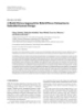
Báo cáo hóa học: "Review Article A Model-Driven Approach for Hybrid Power Estimation in Embedded Systems Design"
15 p | 49
| 8
-

Báo cáo hóa học: " Review Article AVS-M Audio: Algorithm and Implementation"
16 p | 50
| 8
-
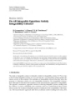
Báo cáo hóa học: " Review Article Do All Integrable Equations Satisfy Integrability Criteria?"
16 p | 47
| 7
-
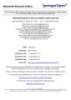
Báo cáo sinh học: "This peer-reviewed article was published"
15 p | 35
| 6
-

Báo cáo hóa học: " Review Article An Overview on Wavelets in Source Coding, Communications, and Networks"
27 p | 54
| 6
-
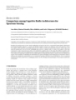
Báo cáo hóa học: " Review Article Comparison among Cognitive Radio Architectures for Spectrum Sensing"
18 p | 47
| 6
-

Báo cáo hóa học: " Review Article q-Genocchi Numbers and Polynomials Associated with q-Genocchi-Type l-Functions"
12 p | 63
| 6
-
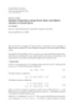
Báo cáo hóa học: " Review Article Remarks of Equivalence among Picard, Mann, and Ishikawa Iterations in Normed Spaces Xue Zhiqun"
5 p | 47
| 5
-
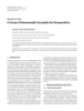
Báo cáo hóa học: " Review Article A Survey of Homomorphic Encryption for Nonspecialists"
10 p | 44
| 5
-
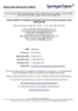
Báo cáo sinh học: " This peer-reviewed article was published immediately upon acceptance. It can be downloaded, printed "
16 p | 57
| 5
-

Báo cáo hóa học: " Research Article A Review of Signal Subspace Speech Enhancement and Its Application to Noise Robust Speech Recognition
15 p | 57
| 5
-
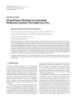
Báo cáo hóa học: " Review Article Bit and Power Allocation in Constrained Multicarrier Systems: The Single-User Case"
14 p | 55
| 4


Chịu trách nhiệm nội dung:
Nguyễn Công Hà - Giám đốc Công ty TNHH TÀI LIỆU TRỰC TUYẾN VI NA
LIÊN HỆ
Địa chỉ: P402, 54A Nơ Trang Long, Phường 14, Q.Bình Thạnh, TP.HCM
Hotline: 093 303 0098
Email: support@tailieu.vn
Giấy phép Mạng Xã Hội số: 670/GP-BTTTT cấp ngày 30/11/2015 Copyright © 2022-2032 TaiLieu.VN. All rights reserved.

