


Lecture Advanced Econometrics (Part II) - Chapter 10: Models for panel data
lượt xem 2
download
 Download
Vui lòng tải xuống để xem tài liệu đầy đủ
Download
Vui lòng tải xuống để xem tài liệu đầy đủ
Lecture "Advanced Econometrics (Part II) - Chapter 10: Models for panel data" presentation of content: General framework for panel data, pooled regression, fixed effects, random effects model, choosing between fixed and random effects models, finding big.
Bình luận(0) Đăng nhập để gửi bình luận!
Nội dung Text: Lecture Advanced Econometrics (Part II) - Chapter 10: Models for panel data
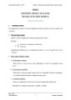
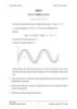
- Advanced Econometrics Chapter 10: Models for panel data Chapter 10 MODELS FOR PANEL DATA I. GENERAL FRAMEWORK FOR PANEL DATA Panel data (longitudinal data): same entities are observed overtime. The basic framework for panel data is a regression model of the form: k (1) Yit = ∑ β j X itj + ziα + ε it j =1 (1×l )( l ×1) = X it β + ziα + ε it (1× k )( k ×1) (1×l )( l ×1) Where: zi = [1 zi 2 ... zil ] α1 α α = 2 ... αl X it = [ X it1 X it 2 ... X itk ] There are k regressors in X it , not including a constant term. The heterogeneity or individual effect is ( ziα ) where zi contains a constant term and a set of individual or group specific variable, which may be observed, such as race, sex, location,… or unobserved, such as family specific characteristics, individual heterogeneity in skill or preferences,… All of which are taken to be constant over time t. Therefore: zi = [1 zi 2 ... zil ] = constant over time t. If zi is observed for all cross-sections (individuals), then the entire model can be treated as an ordinary linear model and fit by least squares. When zi is not observed (most of the cases), complications arise that leads to main objective of the analysis will be consistent and efficient estimation of the partial effects. Nam T. Hoang University of New England - Australia 1 University of Economics - HCMC - Vietnam
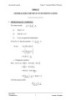
- Advanced Econometrics Chapter 10: Models for panel data ∂E Yit X it β= ∂X it Assumption of strict exogeneity: E ( ε it X i1 , X i 2 ,..., X iT ) = 0 That is, the current disturbance is uncorrelated with the independent variable in every period of t. Assumption of mean independence: ( E zi α X i1 , X i 2 , , X iT l ×1 ) =α 1×1 Or = (fixed effect) = h( X i ) = αi II. POOLED REGRESSION If zi = [1 zi 2 ... zil ] =1, which contains only a constant term. Then OLS provides consistent and efficient estimates of the intercept α and the slope vector β (common effect model). Thus equation (1) → Yit = X it β + ziα + ε it (1× k )( k ×1) (1×l )( l ×1) Where X it it obs of all k explanatory variables: Y1 X 1 i ε1 ( T ×1) ( T ×1) ( T ×1) ( T ×1) Y2 X 2 i ε = β + α + 2 ( k ×1) (1×1) Y X i ε ( T ×N1) ( T ×Nk ) ( T ×1) ( T ×N1) ( NT ×1) ( NT ×1) ( NT ×1) ( NT ×1) 1 1 i = → 1st country: Y1= X 1β + iα + ε1 ( T ×1) 1 E (ε it ) = 0 with classical assumptions: Var (ε it ) = σ ε2 with ∀(i ≠ j ) or (t ≠ s ) Cov (ε , ε ) = 0 it js Nam T. Hoang University of New England - Australia 2 University of Economics - HCMC - Vietnam
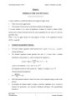
- Advanced Econometrics Chapter 10: Models for panel data III. FIXED EFFECTS 1. Assumption: E ( zi α ) = αi = h( X i ) 1×l l ×1 1×1 Different across units can be captured in differences in the constant term: Yit = X it β + ziα + ε it Yit= X it β + αi + ε it + ( ziα − αi ) υi ( ziα − αi ) = ziα − h( X i ) White noise= Because ziα − h( X i ) is uncorrelated with Xi, we may absorb it in the disturbance: η=i ε it + υi Yit= X it β + αi + ε it Each αi is treated as an unknown parameter to be estimated: i α1 ( T ×1) (1×1) Y = X β + iα 2 + ε ( NT ×1) ( NT ×k ) ( k ×1) ( NT ×1) iα N α1 (1×1) X β + [ d1 d 2 d N ] α 2 + ε = ( NT ×1) ( NT × N ) D α N 1 0 1 0 1 0 0 1 0 1 d1 = di = 0 1 0 0 0 0 0 0 Nam T. Hoang University of New England - Australia 3 University of Economics - HCMC - Vietnam
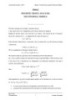
- Advanced Econometrics Chapter 10: Models for panel data α1 ε1 Y1 X 1 i 0 0 ( T ×1) ( T ×1) Y X 0 i 0 α2 ε 2 2 = 2 β + + ( k ×1) α ε YN X N 0 0 i ( T ×N1) ( T ×N1) ( NT ×1) ( NT ×k ) ( NT × N ) ( N ×1) ( NT ×1) Y = X β + D α + ε ( NT ×1) ( NT ×k ) ( k ×1) ( NT × N ) ( N ×1) ( NT ×1) This model is also called “Least Squares Dummy Variables” (LSDV) because it can be estimated directly with the intercept dummies. 2. The Within-Groups and Between-Groups Estimators There are 3 ways to estimate the pooled regression model: α X it β + ε it Yit =+ Using OLS: −1 N T N T → βˆOLS = ∑∑ ( X it − X ) '( X it − X ) ∑∑ ( X it − X ) '(Yit − Y ) ( k ×1) =i 1 =t 1 =i 1 =t 1 Note: ( X it − X ) and ( X it − X ) ' (1×k ) ( k ×1) X and Y are overall means: (1×k ) ( k ×1) 1 X = ∑∑ X it (1×k ) (1×k ) NT 1 Y = ∑∑ Yit ( k ×1) ( k ×1) NT Using the deviation from the group means Yit − Yi . =α + X it − X i . β + ( ε it − ε i . ) ( k ×1) (1×k ) (1×k ) ( k ×1) We get the Within – Group estimator: −1 N T N T → βˆLSDV = βˆwithin= ∑∑ ( X it − X i . ) '( X it − X i . ) ∑∑ ( X it − X i . )(Yit − Yi . ) ( k ×1) =i 1 =t 1 =i 1 =t 1 This is also the LSDV or fixed effect estimator of 𝛽 Nam T. Hoang University of New England - Australia 4 University of Economics - HCMC - Vietnam
- Advanced Econometrics Chapter 10: Models for panel data 1 T (1×k ) ∑ X i. = T t =1 X it Where T group means. (i = 1, 2, ..., N) Yi . = ∑ Yit 1 (1×1) T t =1 We can write the model in terms of the group means: α X i.β + ε i. Yi . =+ (i = 1, 2, ..., N) We use only N observations, (the group means). Apply OLS to N observations, we get the Between – Group estimator: −1 N N → βˆBetween = ∑ ( X i . − X ) '( X i . − X ) ∑ ( X i . − X )(Yi . − Y ) i =1 i =1 Back to the fixed effects: = [X ' MDX ] [ X ' M DY ] −1 → βˆFE where M D= I − D ( D ' D ) −1 D ' M 0 0 0 0 M0 0 MD = 1 M= 0 IT − ii ' T 0 0 M 0 VarCov ( βˆFE ) = σˆ 2 [ X ' M D X ] −1 σˆ= 2 1 Y − M D X βˆ ′ Y − M D X βˆ NT − N − K Note: Why pooled estimator, within group estimator and between group estimator are different? Because: N T 2 • Pooled estimator: Min βˆ pooled ∑∑ eit =i 1 =t 1 N T • Within-group estimator: Min β within ˆ ∑∑ =i 1 =t 1 ( eit − ei . ) 2 N T • Between-group estimator: Min βˆbetween ∑∑ =i 1 =t 1 ( ei . ) 2 There are 3 different minimum problems, eit are the same from: Nam T. Hoang University of New England - Australia 5 University of Economics - HCMC - Vietnam
- Advanced Econometrics Chapter 10: Models for panel data α X it βˆ + eit Yit =+ eit = Yit − α − X it βˆ Note that in deviation form: (Yi − Y )= (X i − X ) βˆ + ei − ei and Yi =+ α X i βˆ + ei , βˆ and ei are the same. 3. Fixed time and Group Effects The LSDV approach can be extended to include a time specific effect as well: Yit= X it β + αi + γ t + ε it α1 γ 2 α γ X it β + d it1 d it2 d itN 2 + git2 Yit = git3 gitT 3 + ε it α N γ T (one of the time effects must be dropped to avoid perfect co linearity – the group effects and time effects both sum to one) 1 if i = j 1 if t = s d = j it any t gits = any i 0 if not 0 if not For panel data now we can use • Pooled • Fixed effects o Time effects only o Group effects only o Time and group effect 4. Unbalanced Panel: −1 −1 N Ti N Ti βˆLSDV = βˆFE = β within= ∑ ∑ ( X it − X i . ) '( X it − X i . ) ∑ ∑ ( X it − X i . ) '(Yit − Yi . ) ˆ ( k ×1) i1 i 1= = = i1 i 1= 5. Allow for autocorrelation and heteroskedasticity in error term: =ε it ρ iε i ,t −1 + uit ρi < 1 Nam T. Hoang University of New England - Australia 6 University of Economics - HCMC - Vietnam
- Advanced Econometrics Chapter 10: Models for panel data E (uit ) = 0 E (uit uis ) = 0 for t ≠ s (no temporal auto in uit) E (uit u jt ) = 0 for i ≠ j (no spatial auto) E (uit u js ) = 0 for i ≠ j and t ≠ s E (uit2 ) = σ 2 i = 1, 2, ..., N (spatial heteroskedasticity but no temporal auto) Estimation: • Estimate (1) by OLS → get eit's T ∑e e it it −1 • ρˆ = t =2 T for i = 1, 2, ..., N (use all NT observations). ∑e t =2 2 it −1 n 1 or ρˆ = N ∑ ρˆ i =1 i if T is small. • Use ρˆi 's to quasi-difference (1): (Yit − ρˆiYit −1 ) = ( X it − ρˆi X it −1 ) β + α (1 − ρˆi ) + ( ε it − ρˆiε it −1 ) ≈uit Estimate by OLS with N(T-1) observations → uˆit T T ∑ uˆit2 ∑ uˆ 2 it • σˆ u2 = t =2 or σˆ u2i = t =2 i T −1− k T −1 • From WLS: Yit* X it* 1 − ρ i uit = β + α + σˆ ui σˆ ui σˆ ui σˆ ui OLS → estimator ⇒ BLUE 6. Testing for Group - Special Effects: The standard F test can be used to test whether the pooled or fixed-effect model is more appropriate: H0: C= 1 C= 2 = C N= α Ci = ziα * Nam T. Hoang University of New England - Australia 7 University of Economics - HCMC - Vietnam
- Advanced Econometrics Chapter 10: Models for panel data 2 ( RLSDV − R pooled 2 ) ( N − 1) F F ( N − 1, NT − N − k ) (1 − R 2 LSDV ) ESSU ( NT − N − k ) 7. Shortcoming of the fixed effects: The coefficients on the time-invariant variables cannot be estimated by within estimators. IV. RANDOM EFFECTS MODEL: 1. Model: Yit = X it β + ziα * + ε it Denote: ziα * = ci Fixed effects assume ci are correlated with Xi E ( ci X i ) = h( X i ) = αi 1×1 Random effects assume ci are uncorrelated with Xi E ( ci X i ) = α = constant. → c= i α + ui with ui ∼ iid. then Yit= X it β + (α + ui ) + ε it =α + X it β + (ui + ε it ) (ci and Xi are not correlated). The following assumptions are made: E (ε it X )=0 E (uit X )=0 ( NT ×k ) ( NT ×k ) E (ε it2 ) = σ ε2 E (uit2 ) = σ u2 E (ε itε js ) = 0 for i ≠ j or t ≠ s or both. E (ui u j ) = 0 for i ≠ j E (uiε js ) = 0 for all i,j,s Let: ηit= ui + ε it E (ηit2 ) =E (ui + ε it ) 2 =σ u2 + σ ε2 E (ηitη jt ) = E (ui + ε it )(u j + ε jt ) = 0 Nam T. Hoang University of New England - Australia 8 University of Economics - HCMC - Vietnam
- Advanced Econometrics Chapter 10: Models for panel data E (ηitηis ) = E (ui + ε it )(ui + ε is ) = σ u2 Y= X β + η ( NT ×1) ( NT ×1) η1 η 2 η = ( NT ×1) (ηT ×N1) ( NT ×1) σ u2 + σ ε2 σ u2 σ u2 σ u2 σ u2 + σ ε2 σ u2= Σ E (ηη i j) = ' ( T ×T ) (T ×T ) 00 σu σ u2 σ u2 + σ ε2 2 E (ηη i j) = 0 ' ( T ×T ) ( T ×T ) So: Σ00 0 0 0 Σ00 0 = E (ηη Σ = ' ) ( NT × NT ) i j ( NT × NT ) 0 0 Σ00 We can estimate βˆRE by GLS estimation: βˆRE ( X ' Σ −1 X ) −1 ( X ' Σ −1Y ) = ( k ×1) = ( X *' X * ) −1 ( X *'Y* ) = [( PX ) '( PX )] [( PX ) '( PY )] −1 Σ00 −1/2 0 0 −1/2 0 Σ 0 P ' P = Σ −1 → −1/2 P= I N ⊗ Σ00 = 00 −1/2 0 0 Σ00 −1/2 1 θ ' Σ00 = I T − iT iT σε T σε θ = 1− σ ε + T σ u2 2 Yi1 − θ Yi . 1 Yi 2 − θ Yi . Y*i = and the same for X*i σε YiT − θ Yi . Nam T. Hoang University of New England - Australia 9 University of Economics - HCMC - Vietnam
- Advanced Econometrics Chapter 10: Models for panel data 2. Feasible Estimation: We need to estimated σ ε2 and σ u2 Estimation of σ ε2 : Yit =α + X it β + (ui + ε it ) → Yi . =α + X i . β + (ui + ε i . ) → (Y it − Yi . ) = (X it − X i . ) β + (ε it + ε i . ) (*) Estimate (*) using OLS and use the residuals to get the estimation of σ ε2 N T ∑∑ (e it − ei . ) 2 σˆ ε2 = =i 1 =t 1 NT − N − k Estimation of σ u2 : (ui + ε i . ) = Yi . − α − X i . β e* σ ε2 Var (ui + ε i . ) = σ u2 + T e*' e* σˆ Estimation of Var (ui + ε i . ) is − ε N −k T Insert σ ε2 , σ u2 into Σ and calculate βˆRE V. CHOOSING BETWEEN FIXED AND RANDOM EFFECTS MODELS: Whether ci = ziα * are correlated with (Xi) or not. If they are → RE will produce inconsistent estimates. If they are not → RE model may be preferable. 1. Think through the problem: 2. Hausman Specification Test: ( ′ ) ( ) ( ) ( ) −1 βˆwithin − βˆRE Var βˆwithin − Var βˆRE βˆwithin − βˆRE χ (2k −1) W= H0: no correlation between Ci and Xi HA: correlation between Ci and Xi Nam T. Hoang University of New England - Australia 10 University of Economics - HCMC - Vietnam
- Advanced Econometrics Chapter 10: Models for panel data Under H0: Both βˆFE and βˆRE are consistent estimators but only βˆRE is efficient. VI. FINDING BIG Σ: Example 1: =ε it ρ iε i ,t −1 + uit ρi < 1 E (uit ) = 0 E (uit2 ) = σ u2i E (ε itε jt ) = 0 E (ε itε is ) = 0 for t ≠ s (no temporal auto) E (ε itε js ) = 0 for t ≠ s (no temporal auto) ε1 ( T ×1) ε ε = 2 ε ( T ×N1) ( NT ×1) Σ = E (εε ') off-diagonal blocks t ≠ s : E ( ε i ε j ' ) = 0 ( T ×1) ( T ×1) diagonal blocks 1 ρi ρ i2 ρ iT −1 ρ 1 ρ i2 ρ iT −2 E( εi εi = ') i = σ ε2i Ω ( T ×1) ( T ×1) ( T ×T ) T −1 ρi ρ ρ T −2 T −3 i i 1 σ ε21 Ω1 0 0 0 σ ε2 Ω2 2 0 σˆ u2i E (εε ′) = σ = ˆ 2 ( NT × NT ) with εi 1 − ρˆi2 0 0 σ ε2N Ω N Example 2: Now assume no temporal autocorrelation. But allow spatial autocorrelation and cross-section heteroskedasticity. E (uit ) = 0 E (uit2 ) = σ u2i Nam T. Hoang University of New England - Australia 11 University of Economics - HCMC - Vietnam
- Advanced Econometrics Chapter 10: Models for panel data E (ε itε jt= ) σ ij ≠ 0 spatial autocorrelation E (ε itε is ) = 0 for t ≠ s (no temporal auto) E (ε itε js ) = 0 for t ≠ s (no temporal auto) Σ = E (εε ') ε1 ( T ×1) ε ε = 2 ε ( T ×N1) ( NT ×1) Same country: σ ii 0 0 0 σ 0 =E (εε ′) = ii σ ii I ( NT × NT ) 0 0 σ ii Different country i ≠ j : σ ij 0 0 0 σ 0 =E ( ε i ε j ' ) = σ I ij ( T ×1) ( T ×1) ij 0 0 σ ij σ 11 I σ 12 I σ 1N I σ I σ I σ 2N I E (εε ′) = 21 22 ( NT × NT ) σ N 1 I σ N 2 I σ NN I Nam T. Hoang University of New England - Australia 12 University of Economics - HCMC - Vietnam
CÓ THỂ BẠN MUỐN DOWNLOAD
-
Lecture Advanced Econometrics (Part II) - Chapter 3: Discrete choice analysis - Binary outcome models
 18 p |
  61
|
61
|  6
6
-
Lecture Advanced Econometrics (Part II) - Chapter 13: Generalized method of moments (GMM)
9 p | 83
| 4
-

Lecture Advanced Econometrics (Part II) - Chapter 5: Limited dependent variable models - Truncation, censoring (tobit) and sample selection
13 p | 61
| 4
-
Lecture Advanced Econometrics (Part II) - Chapter 6: Models for count data
7 p | 78
| 3
-
Lecture Advanced Econometrics (Part II) - Chapter 4: Discrete choice analysis - Multinomial models
13 p | 71
| 3
-

Lecture Advanced Econometrics (Part II) - Chapter 6: Dummy varialable
0 p | 70
| 2
-
Lecture Advanced Econometrics (Part II) - Chapter 2: Hypothesis testing
7 p | 54
| 2
-
Lecture Advanced Econometrics (Part II) - Chapter 7: Greneralized linear regression model
0 p | 63
| 2
-
Lecture Advanced Econometrics (Part II) - Chapter 8: Heteroskedasticity
0 p | 102
| 2
-
Lecture Advanced Econometrics (Part II) - Chapter 9: Autocorrelation
0 p | 44
| 2
-

Lecture Advanced Econometrics (Part II) - Chapter 11: Seemingly unrelated regressions
0 p | 71
| 2
-

Lecture Advanced Econometrics (Part II) - Chapter 12: Simultaneous equations models
0 p | 73
| 2
-
Lecture Advanced Econometrics (Part II) - Chapter 1: Review of least squares & likelihood methods
6 p | 64
| 2


Chịu trách nhiệm nội dung:
Nguyễn Công Hà - Giám đốc Công ty TNHH TÀI LIỆU TRỰC TUYẾN VI NA
LIÊN HỆ
Địa chỉ: P402, 54A Nơ Trang Long, Phường 14, Q.Bình Thạnh, TP.HCM
Hotline: 093 303 0098
Email: support@tailieu.vn
Giấy phép Mạng Xã Hội số: 670/GP-BTTTT cấp ngày 30/11/2015 Copyright © 2022-2032 TaiLieu.VN. All rights reserved.

