


Lecture Advanced Econometrics (Part II) - Chapter 12: Simultaneous equations models
lượt xem 2
download
 Download
Vui lòng tải xuống để xem tài liệu đầy đủ
Download
Vui lòng tải xuống để xem tài liệu đầy đủ
Lecture "Advanced Econometrics (Part II) - Chapter 12: Simultaneous equations models" presentation of content: Model, rank and order conditions for identification, estimation of a simultaneous equation system.
Bình luận(0) Đăng nhập để gửi bình luận!
Nội dung Text: Lecture Advanced Econometrics (Part II) - Chapter 12: Simultaneous equations models
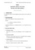
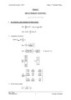
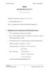
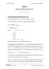
- Advanced Econometrics Chapter 12: Simultaneous equations models Chapter 12 SIMULTANEOUS EQUATIONS MODELS I. MODEL: Many economic problems involve the interaction of multiple endogenous variables within a system of equations. Estimating the parameters of such as system is typically not as simple as doing OLS equation-by-equation. Issues such as identification (wether the parameters are even estimable) and endogeneity bias are then primary topic in this chapter. 1. Example: Demand and supply for peanuts at t q=d ,t α pt + ε1t qs ,t = β pt + γ Rt + ε 2 t qt = quantity, pt = price, Rt = input price. Equilibrium: qd,t = qs,t = qt ⇔ α pt + ε1t = β pt + γ Rt + ε 2 t ⇔ (α − β ) pt = γ Rt + ε 2 t − ε1t γ ε 2 t − ε1t ⇔ = pt Rt + (α − β ) (α − β ) The model is the joint determination of price and quantity qt and pt are endogenous variables, Rt is assume determined outside the model, it is exogenous variable. All three equations are needed to determine the equilibrium price and quantity. Note: The completeness of the system requires that the number of the equations equals the number of endogenous variables. 2. General model: The simultaneous system can be written as: Nam T. Hoang University of New England - Australia 1 University of Economics - HCMC - Vietnam
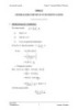
- Advanced Econometrics Chapter 12: Simultaneous equations models Y t Γ + X t Β + εt =0 (1× M ) ( M × M ) (1× K ) ( K × M ) (1× M ) Where: Yt = [Y1 Y2 YM ]t X t = [ X1 X 2 X M ]t ε t = [ε1 ε 2 ε M ]t γ 11 γ 12 γ 1M γ γ 22 γ 2M Γ = 21 ( M ×M ) γ M 1 γ M 2 γ MM β11 β12 β1M β β 22 β2M Β = 21 ( M ×M ) βM1 βM 2 β KM α1 + β11 pt + β12 I t + β13 pt* + ε1t qt = α 2 + β 21 pt + ε 2 t qt = It: Income; pt* : price of an alternative; qt, pt: Endogenous (determined within the model) It, Rt, pt* : Exogenous (determined outside the model) Matrix form: +α1 +α 2 −1 −1 * [ qt pt ] + 1 I t pt + β12 0 + [ε1t ε 2 t ] = [0 0] + β11 + β 21 Yt Xt + β13 0 εt Γ Β 3. Reduced form: Each endogenous variable is expressed in terms of all exogenous variables: Yt= X t Π + Vt Where: Π =− Β Γ −1 ( K ×M ) ( K ×M ) Nam T. Hoang University of New England - Australia 2 University of Economics - HCMC - Vietnam
- Advanced Econometrics Chapter 12: Simultaneous equations models = Vt ε t Γ −1 (1× M ) (1× M ) ( M × M ) If the system is completeness → Γ squared matrix is non-singular and Γ−1 exists. π 11 π 12 = qt pt ] 1 I t p π 21 π 22 + [V1t V2 t ] [ * t Yt Xt π 31 π 32 • Reduced form can always be estimated, so reduced form equations are identified. • If πij are given we can find structural parameters: π 11 π 12 +α1 +α 2 −1 −1 ΠΓ = −Β ⇔ π 21 π 22 = − + β12 0 + β11 + β 21 π 31 π 32 + β13 0 Γ Β For equation (1): demand −π 11 + π 12 β11 = −α1 −π 21 + π 22 β11 =− β12 −π + π β = − β13 31 32 11 This is “Indirect least squares” estimation (ILS) Over-identification → ILS cannot be applied? ⇒ 3 equations, 4 unknown: β11 , α1 , β12 , β13 . So parameters of 1st structure equation (demand) are not identified. This equation cannot be estimated. For equation (2): supply −π 11 + π 12 β 21 = −α 2 β 21 = π 21 / π 22 −π 21 + π 22 β 21 =0 ⇒ −π + π β = α π 11 − π 12 (π 21 / π 22 ) = 31 32 21 0 II. RANK AND ORDER CONDITIONS FOR IDENTIFICATION: 1. Classification of variables: + Current endogenous (unlagged) = jointly dependent + Predetermined: a. Exogenous (unlagged & lagged) Nam T. Hoang University of New England - Australia 3 University of Economics - HCMC - Vietnam
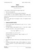
- Advanced Econometrics Chapter 12: Simultaneous equations models b. Lagged endogenous Ex: variables qt −1 or pt −1 on RHS equation Notation: for a given equation M* = number of endogenous variables in this equation M** = number of endogenous variables in system (excluded) K* = number of included predetermined variables in this equation KK* = number of excluded M = M ∗ + M ∗∗ ; K = K ∗ + K ∗∗ 2. Order conditions: Yt Γ + X t Β + ε t = 0 Yt = − X t ΒΓ −1 − ε t Γ −1 = 0 Y + X t Π + Vt t (1× M ) (1× K ) ( K × M ) (1× M ) Π =− Β Γ −1 ( k ×M ) ( K ×M ) Π can be known by OLS because reduced form always identified. Question: Can β ij 's and γ ij 's (Β and Γ) be fund in terms of Π ij 's (Π) We have: Π = −ΒΓ −1 ⇒ ΠΓ = −Β ⇒ ΠΓ + Β = 0 Γ ⇒ ( KΠ×M ) ( KI×KM ) Β = 0 ( K ×M ) K ×( M + K ) A ( M +K )M Consider the first equation: Nam T. Hoang University of New England - Australia 4 University of Economics - HCMC - Vietnam
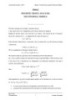
- Advanced Econometrics Chapter 12: Simultaneous equations models γ 1 ⇒ [ Π IK ] = 0 β1 ( K ×1) K ×( M + K ) A ( M + K )1 We have K equations, K+M unknown variables → It is impossible to be identification without additional information. ∗ Theorem: A necessary condition for a given equation to be identified is that the number of predetermined variables excluded (K**) from this equation be greater than or equal to the number of jointly dependent variables included in this equation mins 1. K ** ≥ M * − 1 K ** + M ** ≥ M * + M ** − 1 K ** + M ** ≥ M − 1 Excluded variables # Dependent variables in system -1 Ex. Demand: K ** = 0 M *= 2 − 1= 1 ⇒ not identified pt ,qt Supply: K ** = 2 M *= 2 − 1= 1 ⇒ order condition is satisfied, not identified yet. I t , Pt* pt ,qt If over identified: K ** > M * − 1 If exactly identified: K= ** M * −1 3. Rank conditions: γ 1 [ Π IK ] = 0 β1 ( K ×1) K ×( M + K ) ( M + K )×1 a K equations, (M + K) unknown parameters Added information in the form of general linear restrictions on a : R1a1 = 0 R1 a1 ( r1 ×1) r1 ×( M + K ) [ r1 ×( M + K )] [( M + K )×1] r1: number of restrictions on exogenous & endogenous variables. Nam T. Hoang University of New England - Australia 5 University of Economics - HCMC - Vietnam
- Advanced Econometrics Chapter 12: Simultaneous equations models 0 0 1 0 0 0 1 1 1 1 = R1 3rd coefficient = 0, sum of coefficients on variables 2 → 5 = 0. M K γ 1 Π R I K = K 0 β1 ( r1 + K )×1 r1 1 ( r1 + K )×( M + K ) ( M + K )×1 a ∗ Theorem: A necessary and sufficient condition for a solution a to this system of homogenous Π IK equations is that the rank of K be equals to (M + K – 1) this solution is nontrivial R1 and unique up to a factor of proportionality. ∗ An equivalent condition is that the rank of: (R1A) = M - 1 Π IK Because Rank ( R1 A) + K = Rank R1 • Rank condition: necessary and sufficient condition for identification: Rank ( R1 A= ) M −1 • Order condition: necessary: r1 ≥ M − 1 Number of rows of R1 is a number of endogenous variables and exogenous variables outside the equation (1) K** + M** → order condition now: r1 ≥ M − 1 : Y1t= γ 11Y2 t + γ 12Y3t + β11 + β12 X 2 t + ε1t Y2 t = + γ 22Y3t + β 21 + β 22 X 2 t + β 23 X 3t + ε 2 t =Y3t γ 31Y2 t + β 31 + β 32 X 2 t + β 33 X 3t + ε 3t ( β 32 = β 33 ) Yjt: endogenous variables, Xjt: Exogenous (predetermined) Matrix form: Nam T. Hoang University of New England - Australia 6 University of Economics - HCMC - Vietnam
- Advanced Econometrics Chapter 12: Simultaneous equations models β11 β 21 β 31 −1 0 0 β 0 Y3t ] γ 11 −1 γ 31 + [1 X 1t 0 [Y1t Y2 t X 2t X 3t ] 12 0 β 22 β 32 γ 12 γ 21 −1 0 β 23 β 33 + [ε1t ε 2 t ε 3t ] = [0 0 0] • For equation (1): write restrictions as: R1a1 = 0 Γ Where a1 is the first column of = A . Then: Β 0 0 1 0 R1 = [ 2×( K + M )] 0 0 0 1 r1 = 2 ≥ M − 1 = 3 − 1 = 2 ⇒ Order condition: yes. 0 β 22 β 32 ( R1 A) = β 33 Rank condition: yes 0 β 23 Rank ( R1 A)= 2= M − 1 → eq(1) is identified. • For equation (2): write restrictions as: R2a2 = 0 1 0 0 0 0 0 0 R2 = 0 0 0 0 1 0 0 r2 = 2 ≥ M − 1 = 3 − 1 = 2 ⇒ Order condition: yes. −1 0 0 Rank condition: yes ( R2 A) = β12 0 0 Rank ( R2 A) =1 ≠ M − 1 → eq(2) is not identified. • For equation (3): ( β 32 = β 33 ) R3a3 = 0 . Then: 1 0 0 0 0 0 0 R3 = 0 0 0 0 1 0 0 0 0 0 0 0 1 −1 Nam T. Hoang University of New England - Australia 7 University of Economics - HCMC - Vietnam
- Advanced Econometrics Chapter 12: Simultaneous equations models r3 = 3 ≥ M − 1 = 2 ⇒ Order condition: yes. −1 0 0 Rank condition: yes ( R3 A) = β12 0 0 (0 − 0) ( β 22 − β 23 ) ( β 32 − β 33 ) Rank ( R3 A)= 2= M − 1 → eq(3) is identified. Example 2: I t =α 0 + α1 (Yt − Yt −1 ) + α 2it + ε1t Ct =β 0 + β1Yt + ε 2 t Yt = Ct + I t + ε 3t Matrix form: −1 0 1 α 0 β 0 0 [ It Ct Yt ] 0 −1 1 + [1 it Yt −1 ] α 2 0 0 + [ε1t [0 0 0] ε 2 t ε 3t ] = α1 β1 −1 α 3 0 0 • For equation (1): r1 = 2 = M − 1 = 3 − 1 = 2 ⇒ Order condition: yes. 0 1 0 0 0 0 R1 = 0 0 1 0 0 1 0 −1 1 0 −1 1 = Rank condition: yes ( R1 A) = (α1 + α 3 ) ( β1 + 0) ( −1 + 0) 0 β1 −1 Rank ( R1 A)= 2= M − 1 → eq(1) is identified. • For equation (2): write restrictions as: R2a2 = 0 r2 =3 ≥ M − 1 ⇒ Order condition: yes. −1 0 1 Rank condition: ( R2 A) = α 2 0 0 A α 3 0 0 Nam T. Hoang University of New England - Australia 8 University of Economics - HCMC - Vietnam
- Advanced Econometrics Chapter 12: Simultaneous equations models Rank ( R1 A)= 2= M − 1 → eq(1) is identified. • For equation (3): r3 = 3 ≥ M − 1 = 2 ⇒ Order condition: yes. Rank ( R3 A)= 2= M − 1 → eq(3) is identified. III. ESTIMATION OF A SIMULTANEOUS EQUATION SYSTEM: 1. Under-identified: Order or rank condition fails. 2. Identified: • Exactly identified: r = M – 1 and rank condition is met. • Over-identified: r > M – 1 and rank condition is met. Problem: How do we estimate Β, Γ consistently? a) If a system is under-identified (there are some equations which are under-identified) → there is no way to estimate it consistently. b) If a system is exact-identified: One possible way is to use indirect least squares estimation to solve. Π IK γ R = 0 1 β c) If a system is over-identified: ILS does not work because there will be more than one possible estimator and no obvious means of choosing among them. OLS → inconsistent estimators because of edogeneity, also call: “Simultaneous equation bias” of least squares. We will discuss various methods of consistent and efficient estimation (“All of methods in general use can be placed under the umbrella of instrument variable (I.V) estimator” Greene). Nam T. Hoang University of New England - Australia 9 University of Economics - HCMC - Vietnam
- Advanced Econometrics Chapter 12: Simultaneous equations models ∗ Note: generalised I.V estimator of β: −1 βˆIV = X / M Z X X / M Z Y where M Z = Z ( Z / Z ) −1 Z / Z are instrumental variable for X with L > k. ( n× L ) ( n×k ) If L = k → Z/X is a squared matrix and: (Z X ) −1 −1 =βˆIV = X / M Z X X / M Z Y / Z /Y where M Z = Z ( Z / Z ) −1 Z / (simple IV). −1 And βˆIV = X / M Z X X / M Z Y is also the 2SLS (two-stage least square) estimator: • First stage: get Xˆ = Z Π with Π =( Z / Z ) −1 ZX → Xˆ = Z ( Z / Z ) −1 ZX −1 −1 • Second stage: βˆ2 SLS = Xˆ / Xˆ Xˆ /Y = X / M Z X X / M Z Y = βˆIV when use Xˆ as an IV. We can prove that βˆIV generalized is a consistent estimator of β. −1 βˆIV = X / M Z X X / M Z Y −1 1 / 1 / −1 1 / 1 / 1 / −1 1 / β IV= β + X Z Z Z Z X X Z Z Z Z ε ˆ n n n n n n ( ) −1 β + QXZ QZZ So p lim βˆIV = −1 QZX QXZ QZZ −1 β .0 = General IV estimator is also 2SLS estimator. ∗ Requirement: number of instrumental variables has to be larger than number of endogenous variables in the regression (≥) for 2SLS can be applied. General structural model: (1) Yt εt Γ + Xt Β += 0=t 1, 2 , T (1× M ) ( M × M ) (1× K ) ( K × M ) (1× M ) (1× M ) (1’) Y Γ + X Β + E =0 (T × M ) ( M × M ) (T × K ) ( K × M ) (T × M ) (T × M ) (2) E ( ε t ) = 0 (1× M ) (1× M ) Nam T. Hoang University of New England - Australia 10 University of Economics - HCMC - Vietnam
- Advanced Econometrics Chapter 12: Simultaneous equations models ( (3) E ε t/ ε t = ) Σ ( M ×M ) ( M ×M ) ( (4) E ε t/ ε s = 0 ) ( M ×M ) t≠s (no auto) ( M ×M ) (5) E X t/ ε s = 0 Xt predetermined ( k ×1) (1×M ) ( K ×M ) ( (6) E X t/ X t = Σ XX ) finite, non-singular Well-behave data: X →sample statistics converge to corresponding population. 1 (7) p lim ∑ T t X t/ X t = Σ XX ( k ×k ) ( k ×k ) 1 (8) p lim ∑ X t/ ε t = 0 T t ( k ×1) (1×M ) ( k ×M ) 1 (9) p lim ∑ ε t/ ε t = T t ( M ×1) (1×M ) Σ ( M ×M ) (10) Γ is non-singular We can use the set X as instrumental variables for Y • First equation (1st column) Y γ 1* + X β1* + ε1 = 0 (T × M ) ( M ×1) (T × K ) ( K ×1) (T ×1) (T ×1) −1 β1 ( M * − 1) K* ↔ Y γ1 +X ** + ε1 = 0 (M ) M ** 0 0 M + M = * ** M * K + K = ** K ↔ = y1 Y1 γ1 + X 1 β1 + ε1 (T ×1) [T ×( M * −1)] [( M * −1)×1] (T × K * ) ( K * ×1) (T ×1) Nam T. Hoang University of New England - Australia 11 University of Economics - HCMC - Vietnam
- Advanced Econometrics Chapter 12: Simultaneous equations models γ1 =↔ y1 [Y1 X 1 ] β + ε1 (T ×1) Z1 1 (T ×1) [T ×( K * + M * −1)] δ1 ( K * + M * −1) y1 Z1δ1 + ε1 ↔ = (T ×1) (T ×1) a. OLS estimation: δˆ1= ( Z1/ Z1 ) −1 Z1/ y= 1 δ1 + ( Z1/ Z1 ) −1 Z1/ ε1 OLS 1 1 P lim( δˆ1 = ) δ1 + p lim( Z1/ Z1 ) −1 p lim( Z1/ ε1 ) OLS T T 1 / −1 p lim( T Y1 ε1 ) →≠ 0 δ1 + Σ −ZZ1 ≠ δ1 p lim( 1 X / ε ) →= 0 T 1 1 b. Two-stage least squares: Stage 1 (step1): Reduced form equation for Y1: Y1 = y2 y3 yM * [T ×( M * −1)] (T ×1) (T ×1) (T ×1) y= 2 X Π ˆ + Vˆ 2 2 (T ×1) (T × K ) ( K ×1) (T ×1) yˆ 2 ( T ×1) y= 3 X Π ˆ + Vˆ 3 3 (T ×1) (T × K ) ( K ×1) (T ×1) yˆ3 ( T ×1) … yM * = X Π ˆ + Vˆ M* M* Y1 = X Π ˆ XΠ ˆ + Vˆ Vˆ Vˆ ˆ XΠ 2 3 M* 2 3 M* Y1 = X Π ˆ Π ˆ + Vˆ Vˆ Vˆ ˆ Π 2 3 M* 2 3 M* Π ˆ 1 Vˆ1 Nam T. Hoang University of New England - Australia 12 University of Economics - HCMC - Vietnam
- Advanced Econometrics Chapter 12: Simultaneous equations models Y1 = X Π ˆ + Vˆ = Yˆ + Vˆ 1 1 1 (All M* – 1 reduced form equations for Y1 ) All estimated by OLS → X /V= ˆ 0, Yˆ /V= 1 ˆ 0 1 Put expression for Y1 into 1st structural equation: y1 =Y1γ 1 + X 1β1 + ε1 = [Yˆ1 + Vˆ1 ]γ 1 + X 1β1 + ε1 y1 = Yˆ1γ 1 + X 1β1 + Vˆ1γ 1 + ε1 γ =y1 Yˆ1 X 1 1 + (Vˆ1γ 1 + ε1 ) β1 Zˆ1 δ1 y1 = Zˆ1δ1 + (Vˆ1γ 1 + ε1 ) Step 2 (Stage 2): Estimate by OLS: δˆ1 = ( Zˆ1/ Zˆ1 ) −1 (( Zˆ1/ y1 ) = δ1 + ( Zˆ1/ Zˆ1 ) −1 Zˆ1/ (Vˆ1γ 1 + ε1 ) 2 SLS →0 Zˆ1 are instrument instrumental variables of [Y1 X1 ] δˆ1 is consistent. Zˆ1 = W1 → we get the same δˆ1 2 SLS 2 SLS 3. Instrumental variables estimators: Let W1 be a T × ( M * + K * − 1) matrix such that: 1 (1) p lim W1/ Z1 = ΣWZ finite, non-singular T . 1 (1) p lim W1/ ε1 = 0 finite, non-singular T . δˆ1 = (W1/ Z1 ) −1 ((W1/ y1 ) IV −1 1 1 p lim δˆ1 = δ1 p lim W1/ Z1 p lim W1/ ε1 = δ1 IV T T Nam T. Hoang University of New England - Australia 13 University of Economics - HCMC - Vietnam
- Advanced Econometrics Chapter 12: Simultaneous equations models → δˆ1 is consistent. IV Note: we can use W1 = Zˆ1 = Yˆ1 X 1 as an instrumental variables set → get 2-SLS (2-SLS as IV with W1 = Z� 1 ). 4. Indirect least squares: Requires: exactly identified → K= ** M * − 1 or K ** + M ** =M − 1 δˆ1 = ( X 1/ Z1 ) −1 ( X 1/ y1 ) ILS Note: Z 1 X =W1 1 [T ×( K * + M * −1)] [T ×( K * + M * −1)] → same as estimator of δ1 found by algebraically solving for γ�1 and 𝛽̂1from Π �1 Note: 2-SLS as IV with W1 = Zˆ1 = Yˆ1 X 1 δˆ1 = ( Zˆ1/ Z1 ) −1 (( Zˆ1/ y1 ) = ( Zˆ1/ Zˆ1 ) −1 (( Zˆ1/ y1 ) because of orthogonolity condition: IV _ 2 SLS Zˆ1/ Z1 = Zˆ1/ Zˆ1 Note: 2-SLS computational formula Zˆ1 = Yˆ1 X 1 ˆ = X ( X / X ) −1 X /Y Yˆ1 = X Π 1 1 → Zˆ1 = Yˆ1 X 1 = X ( X / X ) −1 X /Y1 X 1 = X ( X / X ) −1 X / [Y1 X1 ] Because: ( X1 X 2 ) = X ( X / X ) −1 X / ( X 1 X 2 ) I = X ( X / X ) −1 X / X 1 X ( X / X ) −1 X / X 2 = ( X / X ) −1 X / [Y1 X 1 ] X ( X / X ) −1 X / Z1 So: Zˆ1 X= Then: δˆ1 = ( Zˆ1/ Zˆ1 ) −1 (( Zˆ1/ y1 ) 2 SLS Nam T. Hoang University of New England - Australia 14 University of Economics - HCMC - Vietnam
- Advanced Econometrics Chapter 12: Simultaneous equations models = ( Z1/ X ( X / X ) −1 X / X ( X / X ) −1 X / Z1 ) −1 ( X ( X / X ) −1 X / Z1 ) −1 y1 = ( Z1/ X ( X / X ) −1 X / Z1 ) −1 ( Z1/ X ( X / X ) −1 X / y1 ) δˆ1 = ( Z1/ M X Z1 ) −1 ( Z1/ M X y1 ) 2 SLS 5. Three-stage Least Squares Estimation: y1 Z1δ1 + ε1 = y2 Z 2δ 2 + ε 2 = Z1 = [Y1 X1 ] … yM Z M δ M + ε M Z M = [YM = XM ] Using SUR framework: Z1 0 0 y1 [T ×( K * + M * −1)] δ1 ε 1 y δ ε 2 = 0 Z2 0 2 + 2 yM 0 0 Z M δ M ε M y Zδ + ε = y= Z δ + ε (TM ×1) (TM ×1) ε1 (T ×1) ε E (εε ′) = 2 ε1 ε 2 ε N ( MT × MT ) (1×T ) (1×T ) ε N (T ×1) σ 11 I σ 12 I σ 1M I σ I σ I σ I = 21 22 2M = Σ ⊗ IT ( M ×M ) σ M 1 I σ M 2 I σ MM I Σ ={σ ij } MM Define: Nam T. Hoang University of New England - Australia 15 University of Economics - HCMC - Vietnam
- Advanced Econometrics Chapter 12: Simultaneous equations models X 0 0 0 X 0 X= = IM ⊗ X (T × K ) 0 0 X Pre-multiply system by X/ (TM × KM ) X / y X / Zδ + X /ε = (*) ( ) E X / εε / X = X / (Σ ⊗ I ) X = [ I ⊗ X / ](Σ ⊗ I )[ I ⊗ X ] = (Σ ⊗ X / X ) Apply GLS to (*): −1 δˆ= 1 ( Z / X (Σ ⊗ X / X ) −1 XZ 3 SLS = ( Z / X (Σ ⊗ X / X ) −1 X / y Σ is estimated by Σˆ =σˆ ij M ×M ei/ e j where σˆ ij = for all i, j pairs and e= i yi − zi δˆi (i = 1, 2,…, M) T 2 − SLS Different way: 1st stage: Perform 2-SLS for each equation of the system. Save ei s (i = 1,2,…, M); e= i yi − zi δˆi (T ×1) (T ×1) (T ×1) 2 − SLS 2nd stage: ei/ e j Estimate Σ by Σˆ =σˆ ij where σˆ ij = for all i, j pairs M ×M T 3rd stage: (1) → y= Z δ + ε (TM ×1) (TM ×1) Estimate δ by using instrumental variable. Nam T. Hoang University of New England - Australia 16 University of Economics - HCMC - Vietnam
- Advanced Econometrics Chapter 12: Simultaneous equations models Zˆ1 0 0 [T ×( K * + M * −1)] Zˆ = 0 Zˆ 2 0 0 0 Zˆ M Where Zˆ1 = Yˆ1 X 1 Zˆ M = YˆM X M −1 and using GLS method: δˆ1 = ( Zˆ / (Σˆ −1 ⊗ I ) Z ( Zˆ / (Σˆ −1 ⊗ I ) y 3 SLS Note: Zˆ1 = X ( X / X ) −1 X / Z1 … Zˆ M = X ( X / X ) −1 X / Z M → Zˆ= / Z / ⊗ X ( X / X ) −1 X / −1 δˆ1 = ( Z / X (Σˆ −1 ⊗ ( X / X ) −1 ) X / Z ( Z / X (Σˆ −1 ⊗ ( X / X ) −1 ) X / y 3 SLS If we use: OLS −1 δˆIV = = Zˆ / Z Zˆ / y is simply equation-by-equation 2SLS. The improvement of 3SLS is using GLS to gain more efficiency, we need to have one more stage → that is calculate Σˆ =σˆ ij M ×M Note: In the 2-SLS procedure: The matrix: Zˆ1 = Yˆ1 X 1 has (M* + K* - 1) columns, all columns are linear function of the K column of X (Because Zˆ1 = X ( X / X ) −1 X / Z1 ). There exist, at most, K linear independent combination of the columns of X. if the equation is not identified then K ** < M * − 1 → K * + K ** < K * + M * − 1 → K < K * + M * −1 Nam T. Hoang University of New England - Australia 17 University of Economics - HCMC - Vietnam
- Advanced Econometrics Chapter 12: Simultaneous equations models but Zˆ1 = Yˆ1 X 1 only has maximum K independent columns. −1 → Zˆ1 will not have full rank, Zˆ1/ Zˆ1 does not exist → 2-SLS estimators cannot compute. If, however, the order condition but not the rank condition is met, then although the 2- SLS estimator can be computed, it is not a consistent estimator. Note: For a system of exactly identified equation: K < K * + M * −1 → X / Z = squared matrix (K×K) i ( K ×T ) (T × K ) −1 δˆi = ( Z i/ X ( X / X ) −1 ) X / Z i ( Z i/ X ( X / X ) −1 ) X / yi 2 − SLS = ( X / Z i ) −1 ( X / X )( Z i/ X ) −1 ( Z i/ X )( X / X ) −1 X / yi = ( X / Z i ) −1 X / yi → δˆi = δˆ when K = K * + M * − 1 for every equation in the system. 2 − SLS ILS Nam T. Hoang University of New England - Australia 18 University of Economics - HCMC - Vietnam
CÓ THỂ BẠN MUỐN DOWNLOAD

-
Lecture Advanced Econometrics (Part II) - Chapter 3: Discrete choice analysis - Binary outcome models
 18 p |
  61
|
61
|  6
6
-
Lecture Advanced Econometrics (Part II) - Chapter 13: Generalized method of moments (GMM)
9 p | 83
| 4
-

Lecture Advanced Econometrics (Part II) - Chapter 5: Limited dependent variable models - Truncation, censoring (tobit) and sample selection
13 p | 61
| 4
-
Lecture Advanced Econometrics (Part II) - Chapter 6: Models for count data
7 p | 78
| 3
-
Lecture Advanced Econometrics (Part II) - Chapter 4: Discrete choice analysis - Multinomial models
13 p | 71
| 3
-

Lecture Advanced Econometrics (Part II) - Chapter 6: Dummy varialable
0 p | 70
| 2
-
Lecture Advanced Econometrics (Part II) - Chapter 2: Hypothesis testing
7 p | 54
| 2
-
Lecture Advanced Econometrics (Part II) - Chapter 7: Greneralized linear regression model
0 p | 63
| 2
-
Lecture Advanced Econometrics (Part II) - Chapter 8: Heteroskedasticity
0 p | 102
| 2
-
Lecture Advanced Econometrics (Part II) - Chapter 9: Autocorrelation
0 p | 44
| 2
-
Lecture Advanced Econometrics (Part II) - Chapter 10: Models for panel data
0 p | 80
| 2
-

Lecture Advanced Econometrics (Part II) - Chapter 11: Seemingly unrelated regressions
0 p | 71
| 2
-
Lecture Advanced Econometrics (Part II) - Chapter 1: Review of least squares & likelihood methods
6 p | 64
| 2


Chịu trách nhiệm nội dung:
Nguyễn Công Hà - Giám đốc Công ty TNHH TÀI LIỆU TRỰC TUYẾN VI NA
LIÊN HỆ
Địa chỉ: P402, 54A Nơ Trang Long, Phường 14, Q.Bình Thạnh, TP.HCM
Hotline: 093 303 0098
Email: support@tailieu.vn
Giấy phép Mạng Xã Hội số: 670/GP-BTTTT cấp ngày 30/11/2015 Copyright © 2022-2032 TaiLieu.VN. All rights reserved.

