


Physical Processes in Earth and Environmental Sciences Phần 3
lượt xem 5
download
 Download
Vui lòng tải xuống để xem tài liệu đầy đủ
Download
Vui lòng tải xuống để xem tài liệu đầy đủ
Chương 3 Ví dụ, một bề mặt đại dương hiện tại mật độ 1 có thể được cho biết "cảm thấy" lực hấp dẫn giảm vì sự nổi tích cực tác dụng lên nó bằng cách nằm dưới nước môi trường xung quanh có mật độ cao hơn một chút.
Bình luận(0) Đăng nhập để gửi bình luận!
Nội dung Text: Physical Processes in Earth and Environmental Sciences Phần 3
- LEED-Ch-03.qxd 11/27/05 3:59 Page 54 54 Chapter 3 differing density does not “feel” the same gravitational that of the ambient lake or marine waters (Fig. 2.12); these attraction as it would if the ambient medium were not are termed turbidity currents (Section 4.12). there. For example, a surface ocean current of density 1 Motion due to buoyancy forces in thermal fluids is may be said to “feel” reduced gravity because of the posi- called convection (Section 4.20). This acts to redistribute tive buoyancy exerted on it by underlying ambient water heat energy. There is a serious complication here because of slightly higher density, 2. The expression for this buoyant convective motion is accompanied by volume reduced gravity, g , is g g( 2 1)/ 2. We noted earlier changes along pressure gradients that cause variations of that for the case of mineral matter, density m, in atmos- density. The rising material expands, becomes less dense, phere of density a, the effect is negligible, corresponding and has to do work against its surroundings (Section 3.4): to the case m a. this requires thermal energy to be used up and so cooling occurs. This has little effect on the temperature of the ambient material if the adiabatic condition applies: the net rate of outward heat transfer is considered negligible. 3.6.3 Natural reasons for buoyancy We have to ask how buoyant forces arise naturally. 3.6.4 Buoyancy in the solid Earth: The commonest cause in both atmosphere and ocean is Isostatic equilibrium density changes arising from temperature variations acting upon geographically separated air or water masses that then interact. For example, over the c.30 C variation in In the solid Earth, buoyancy forces are often due to near-surface air or water temperature from Pole to equa- density changes owing to compositional and structural tor, the density of air varies by c.11 percent and that of changes in rock or molten silicate liquids. For example, the seawater by c.0.6 percent. The former is appreciable, and density of molten basalt liquid is some 10 percent less than although the latter may seem trivial, it is sufficient to drive that of the asthenospheric mantle and so upward the entire oceanic circulation. It is helped of course by movement of the melt occurs under mid-ocean ridges variations in salinity from near zero for polar ice meltwater (Fig. 3.27). However we note that the density of magma is to very saline low-latitude waters concentrated by evapora- also sensitive to pressure changes in the upper 60 km or so tion, a maximum possible variation of some 4 percent. of the Earth’s mantle (Section 5.1). Density changes also arise when a bottom current picks up In general, on a broad scale, the crust and mantle are sufficient sediment so that its bulk density is greater than found to be in hydrostatic equilibrium with the less dense mountain range thickness of iceberg root hir = ri /(rw - ri) hmr ocean, rwrw ri ho o crustal equilibrium crust rc thickness of crustal root, hcr = rc / ( rw – rc ) antiroot har Moho thickness crustal of crustal mantle hcr “root” antiroot, rm har = (rc – rw) /(rm – rc) hir level of buoyancy compensation: all pressures are equal rw Fig. 3.28 Sketches to illustrate the Airy hypothesis for isostasy, analogos to the “floating iceberg” principle.
- LEED-Ch-03.qxd 11/27/05 3:59 Page 55 Forces and dynamics 55 hmr Ocean Nivel del Mar hc Crust Midocean ridge or rift uplift D rc r1 r2 rc r0 Moho 2,900 kg m–3 3,000 kg m–3 Partial melt Mantle rm 3,350 kg m–3 rm > r0 > rc > r1 > r2 Fig. 3.29 Sketches to illustrate the Pratt hypothesis for isostasy. Here topography is supported by lateral density contrasts in the upper mantle (left) and crust (right). crust either “floating” on the denser mantle or supported Ice sheet by a mantle of lower density. This equilibrium state is h0 or termed isostasy; it implies that below a certain depth the structural load mean lithostatic pressure at any given depth is equal. As already noted (Section 3.5.3), above this depth a Lithosphere lateral gradient may exist in this pressure. In the Airy r1 hypothesis, any substantial crustal topography is balanced l by the presence of a corresponding crustal root of the w0 same density; this is the floating iceberg scenario (Fig. 3.28). In the Pratt hypothesis, the crustal topography is due to lateral density contrasts in the upper mantle (at Asthenosphere the ocean ridges) or in separate floating crustal blocks rm (Fig. 3.29). Sometimes the isostatic compensation due to an imposed load like an ice sheet takes the form of a down- Fig. 3.30 Sketch to illustrate the Vening–Meinesz hypothesis for ward flexure of the lithosphere, accompanied by radial isostatic compensation by lithospheric bending and outward flow outflow of viscous asthenosphere (Fig. 3.30). The reverse due to surface loading. process occurs when the load is removed, as in the isostatic rebound that accompanies ice sheet melting. of lithospheric plate at the mid-ocean ridges (Sections 5.1 An important exception to isostatic equilibrium occurs and 5.2). Lithospheric plates are denser than the astheno- when we consider the whole denser lithosphere resting on sphere and hence at the site of a subduction zone, a low- the slightly less dense asthenosphere, a situation forced by angle shear fracture is formed and the plate sinks due to the nature of the thermal boundary layer and the creation negative buoyancy (Fig. 3.27). 3.7 Inward acceleration In our previous treatment of acceleration (Section 3.2), atmosphere allow motion in curved space, with substance we examined it as if it resulted solely from a change in moving from point to point along circular arcs, like the the magnitude of velocity. In our discussion of speed and river bend illustrated in Fig. 3.31. In many cases, where velocity (Section 2.4), we have seen that fluid travels at a the radius of the arc of curvature is very large relative to certain speed or velocity in straight lines or in curved the path traveled, it is possible to ignore the effects of cur- paths. We have introduced these approaches as relevant vature and to still assume linear velocity. But in many to linear or angular speed, velocity, or acceleration. flows the angular velocity of slow-moving flows gives rise Many physical environments on land, in the ocean, and to major effects which cannot be ignored.
- LEED-Ch-03.qxd 11/27/05 3:59 Page 56 56 Chapter 3 Meander bends, R. Wabash, Grayville, Illinois, USA A r = Radius of curvature v r Center of curvature f B u Angular speed, v = df/dt Linear speed, u, at any point along AB = rv 100 m Fig. 3.31 The speed of flow in channel bends. 3.7.1 Radial acceleration in flow bends hence an inward angular acceleration is set up. This inward-acting acceleration acts centripetally toward the virtual center of radius of the bend. To demonstrate this, Consider the flow bend shown in Fig. 3.31. Assume it to refer to the definition diagrams (Fig. 3.32). Water moves have a constant discharge and an unchanging morphology uniformly and steadily at speed u around the centerline at and identical cross-sectional area throughout, the latter a 90 to lines OA and OB drawn from position points A and rather unlikely scenario in Nature, but a necessary restric- B. In going from A to B over time t the water changes tion for our present purposes. From continuity for direction and thus velocity by an amount u uB uA unchanging (steady) discharge, the magnitude of the with an inward acceleration, a u/ t. A little algebra velocity at any given depth is constant. Let us focus on gives the instantaneous acceleration inward along r as surface velocity. Although there is no change in the length equal to u2/r. This result is one that every motorist of the velocity vector as water flows around the bend, that knows instinctively: the centripetal acceleration increases is, the magnitude is unchanged, the velocity is in fact more than linearly with velocity, but decreases with changing – in direction. This kind of spatial acceleration increasing radius of bend curvature. For the case of the is termed a radial acceleration and it occurs in every River Wabash channel illustrated in Fig. 3.31, the curved flow. upstream bend has a very large radius of curvature, c.2,350 m, compared with the downstream bend, c.575 m. 3.7.2 Radial force For a typical surface flood velocity at channel centerline of u c.1.5 m s 1, the inward accelerations are 9.6 · 10 4 and 4.5 · 10 3 m s 2 respectively. The curved flow of water is the result of a net force being set up. A similar phenomena that we are acquainted with is during motorized travel when we negotiate a sharp bend 3.7.3 The radial force: Hydrostatic force imbalance in the road slightly too fast, the car heaves outward on its gives spiral 3D flow suspension as the tires (hopefully) grip the road surface and set up a frictional force that opposes the acceleration. Although the computed inward accelerations illustrated The existence of this radial force follows directly from from the River Wabash bends are small, they create a flow Newton’s Second Law, since, although the speed of pattern of great interest. The mean centripetal acceleration motion, u, is steady, the direction of the motion is con- must be caused by a centripetal force. From Newton’s stantly changing, inward all the time, around the bend and
- LEED-Ch-03.qxd 11/27/05 3:59 Page 57 Forces and dynamics 57 O (b) (a) a r r = Radius of curvature (+ve outward) u = Mean velocity A C A dr uA B u uB a B du u D (c) Hydrostatic gradient = dh/dr D Change in velocity (negative inward) from A to B over C centerline distance dr is: − du = uB/uA. h2 h1 Acceleration, a, over time taken to travel dr is: a = – du/dt. At the limit, as dt goes to 0, since angle a is common: − du/u = dr/r, D C So: du = – udr/r and a = – du/dt = – (u/r)(dr/dt). At the limit, as dt goes to 0, dr/dt = – u and a = – u2/r or, since u = vr, a = – (vr)2/r = – rv2 Fig. 3.32 (a) and (b) To define the radial acceleration acting in curved flow around channel bends; (c) Superelevation of water on the outside of any bend and sectional view of helical flow cell within any bend. Third Law we know this will be opposed by an equal and water is less. This inequality drives a secondary circulation opposite centrifugal (outward acting) force. This tends to of water, outward at the surface and inward at the bottom push water outward to the outside of the bend, causing a (Fig. 3.32c), that spirals around the channel bend and is linear water slope inward and therefore a constant lateral responsible for predictable areas of erosion and deposition hydrostatic pressure gradient that balances the mean cen- as it progresses. The principle of this is familiar to us while trifugal force (Fig. 3.31). Although the mean radial force stirring a cup of black or green tea with tea leaves in the is hydrostatically balanced, the value of the radial force due bottom. Visible signs of the force balance involved are the to the faster flowing surface water (see discussion of inward motion to the center of tea leaves in the bottom of boundary layer flow in Section 4.3) exceeds the hydro- the cup as the flow spirals outward at the surface and down static contribution while that of the slow-moving deeper the sides of the cup toward the cup center point. 3.8 Rotation, vorticity, and Coriolis force push signifies an acceleration arising from a very real force Earth’s rotation usually has no obvious influence on (there are those who doubt the “realness” of the Coriolis motion, that is, motions closely bound to Earth’s surface force, referring to it as a “virtual” or “pseudo-force”). At a by friction, such as walking down the road, traveling by larger scale, the path of slow-moving ocean currents and motorized transport, observing a river or lava flow, and so air masses are significantly and systematically deflected by on. But experience tells us that rotary motion imparts its motion on rotating Earth. Such motions have come under own angular momentum (Section 3.1) to any object, a fact the influence of the Coriolis force, a physical effect caused never forgotten after attempted exit from, or walk onto, a by gradients in angular momentum. rotating roundabout platform; in both cases a sharp lateral
- LEED-Ch-03.qxd 11/27/05 3:59 Page 58 58 Chapter 3 3.8.1 A mythological thought experiment to illustrate Apparent displacement of p1 at latitude, u, during passage in time, t, of Aeolus's wind relative angular motion = ut (Ω sin u t) = (Ω sin u) ut2 Final Initial King Aeolus governed the planetary wind system in Greek target target Arc defining mythology; it was he who gave the bag of winds to position position motion as seen Odysseus. He was ordered by his boss, Zeus, feasting as p by observer 2 p usual at headquarters high above Mount Olympus, to beat moving with 1 up a strong storm wind to punish a naughty minor god- surface from p1 to p2 dess who had fled far to the East in modern day India. Aeolus, who was in Egypt close to the equator at the time r r observing a midsummer solstice, climbed the nearest mountain and pointed his wind-maker exactly East to line defining: (1) distance, r = ut release a great long wind that eventually reached and laid (2) aim from waste to the goddess’s encampment by the River Indus. blowing position Zeus was pleased with the result and rewarded Aeolus with (3) path seen Ω plenty of ambrosia. Some months later another naughty from space goddess fled north from Olympus in the direction of the frozen wastes of Scythia, for some reason (modern day Blowing position wind speed = u Russia). Zeus again instructed Aeolus, now home from his Egyptian expedition, to let loose the punishing wind. Fig. 3.33 The short-lived Aeolus wind-punisher. Aeolus ascended Olympus, pointed his wind-makers exactly North and released another great long wind. (Fig. 3.33). However, to the terrified Scythians looking However, this time, from his vantage point in the clouds South the incoming wind seemed to them to be affected above Olympus, Zeus sees the wind miss his target by a by a mysterious force moving it progressively to their left, considerable margin, devastating a large area of forest well that is, eastward, as it traveled northward. to the East. This happens over and over again. Zeus is We draw the following conclusions: highly displeased and calls an inquest into the sorry state of 1 On a rotating sphere, fixed observers see radial deflections Aeolus’s intercontinental wind punisher, vowing after the of moving bodies largely free from frictional constraints. Such inquest to use Poseidon’s earthquakes for the purpose in deflections involve radial acceleration and a force must be future. responsible. 2 The magnitude of the deflection and the acceleration 3.8.2 The Aeolus postmortem: A logical increases with increasing latitude. conceptual analysis 3 The deflection with respect to the direction of flow is to the right in the Northern Hemisphere and to the left in the Southern. Earth spins rapidly upon its axis of rotation; in other words 4 To observers outside the rotating frame of reference it has vorticity. It has an angular velocity, , of 7.292 10 5 rads 1 about its spin axis that decreases (i.e. Gods) no deflection is visible. 5 For zonal motion at the equator there is no deflection. equatorward as the sine of the angle of latitude. It also has a linear velocity at the equator of about 463 ms 1; this decreases poleward in proportion to the cosine of latitude. 3.8.3 Toward a physical explanation; First, shear Any large, slow-moving object (i.e. slow-moving with vorticity respect to the Earth’s angular speed) not in direct fric- tional contact with a planetary surface and with a merid- Streamline curvature in fluid flow signifies the occurrence ional or zonal motion is influenced by planetary rotation: of vorticity, (eta) (Section 2.4). Clearly, fluid rotation can a curved trajectory results with respect to Earth-bound be in any direction and of any magnitude. Like in consid- observers (Fig. 3.33). The exceptions are purely zonal erations of angular velocity (Section 2.4), the direction in winds along the equator, by chance the first success of question is defined with respect to that of a normal axis to Aeolus. To Aeolus observing the wind from above the plane of rotation, both carefully specified with respect Olympus (i.e. his reference axes were not on the fixed to three standard reference coordinates. Regarding signs Earth surface), it seemed to travel in a straight line
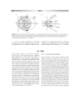
- LEED-Ch-03.qxd 11/27/05 3:59 Page 59 Forces and dynamics 59 Definition of vertical component of vorticity due to horizontal rotation Vertical paddle stick with fins Conventionally +ve anticlockwise zz –ve clockwise Anticlockwise (positive) vertical vorticity contribution 1 u3 +ve u2 +y u1 u1 > u2 > u3 so gradient of u across direction +y is negative, that is, du/dy = –ve Coriolis Anticlockwise (positive) vertical vorticity contribution 2 Fig. 3.34 Vorticity sign conventions and the negative vorticity w3 evident from the flow of Coriolis’s hair. w2 w1 (Fig. 3.34), we define positive cyclonic vorticity with anticlockwise rotation viewed looking down on or into +x the vortical axis; vice versa for negative or anticyclonic w1 < w2 < w3 so gradient of w across direction vorticity. Looked at this way it is clear that vorticity, +x is positive, that is, dw/dx = +ve is a vector quantity; it has both magnitude and direc- tion with vertical, z, streamwise, x, and spanwise, y, Vertical component of vorticity, zz components. Each of these components defines rotation −∂ u /∂ y + ∂ w /∂ x in the plane orthogonal to itself, for example, stream- wise vorticity involves rotations in the plane orthogonal is overall positive to the streamwise direction and since x is the stream- wise component the vorticity refers to rotation in the Fig. 3.35 Shear vorticity and the Taylor vorticity top. plane yz. Now here is the tricky bit (Figs 3.35 and 3.36). In order for rotation to occur there must be a gradient of velocity acting upon a parcel of fluid; if there is no gradient there can be no vorticity. The velocity gradient sets up dw/dx negative or positive gradients of shearing stress and hence this kind of shear +y (w) vorticity (also called relative vorticity) depends upon the magnitude of the gradient, not the absolute velocity of the +x (u) flow itself. This is best imagined by spinning-up a small object, like a top, with one’s fingers to create vertical vor- du/dy ticity (ignore the tendency for precession): a shear couple negative or positive is required from you to turn the object into rotation. Better still for use in flowing fluids, you can make your own vorticity top from a wooden stick and two orthogonal fins (or you can just imagine the vorticity top in a thought experiment). Now, with respect to the plane normal to the vertical spin axis of the vorticity top, only two velocity Fig. 3.36 Combination of velocity gradients that might produce gradients may exist in the xy plane that, between them, overall positive vorticity.
- LEED-Ch-03.qxd 11/27/05 3:59 Page 60 60 Chapter 3 Angular speed of Earth surface is a function of latitude Definition of vertical component of vorticity due r′ to horizontal rotation j f r +ve –ve j>0 j
- LEED-Ch-03.qxd 11/27/05 3:59 Page 61 Forces and dynamics 61 For curved flows we can make use of the coordinate twice the angular velocity, therefore for a given latitude, system shown in Fig. 3.37, with s along the flow direction f 2 sin . With respect to local normal directions from and n in the plane of rotation normal to s and positive the surface, we realize that only at the Pole does the verti- inward toward the center of rotation. V is the local fluid cal vorticity axis align exactly normal to the plane of the speed and r is the radius of the curved flow. The vertical rotation. In fact, vertical vorticity, necessarily defined as vorticity component, z, is now the sum of the shear parallel to the Earth’s axis of rotation, must decrease to ( V/ n) and the curvature (V/r) components, both of zero at the equator when the local normal to the surface is which are positive. in the plane of the rotation. We commonly call Earth’s vorticity, f, the Coriolis parameter. For southern latitudes is taken as negative and thus cyclonic vorticity is nega- 3.8.4 Toward a physical explanation; Second, tive, vice versa for anticyclonic vorticity. The magnitude of solid vortical motions the Coriolis parameter is quite small, of order 10 4 m s 2 between latitudes 45 and 90 . Solid vorticity pertains to solid Earth rotation or to plate and crustal block rotation. It also applies to the rapidly 3.8.5 Finally: Absolute fluid vorticity on rotating cores of tropical cyclones like hurricanes. It is best a rotating Earth investigated initially as curved solid flow, as in the last example (Fig. 3.37), with a rotating disc or turntable Any unbounded fluid, be it water or air, moving slowly setup. In the disc case, both velocity components are gen- over the Earth, must possess not only its own relative or erally nonzero. Consider first the shear term, ( V/ n). shear vorticity, , but also the Earth’s vorticity, f. This is In solid rotation, V r, and the shear term is the absolute vorticity, A, given by the sum, A f. In ( r/ n). Since V is increasing outward with n chosen the slow-moving and slow-shearing oceans, f. Just as positive inward, r/ n 1, the term becomes simply we have to conserve angular momentum so we also have . The contribution, (V/r), due to curvature flow is also to conserve absolute vorticity. The poleward increase in , since V r by definition. Thus for solid body rota- absolute vorticity explains why the slow flows of ocean and tions we have the simple result that the shear and curva- atmosphere are turned by the Coriolis effect, the fluid ture components contribute equally to the total vorticity, motion is turned in the direction of angular velocity and this is equal to 2 . increase as extra angular momentum is obtained from the Now consider the vorticity, f, of a solid sphere like spinning Earth, that is, to the right in the Northern Earth. Viewed from the North Polar rotation axis Hemisphere and to the left in the Southern Hemisphere. (Figs 3.38 and 3.39) Earth spins anticlockwise, with each This, finally, is why earthquakes are better than winds for successive latitude band, , increasing in angular velocity punishing transgressive minor goddesses. poleward by sin . Since the vorticity of a solid sphere is 3.9 Viscosity 3.9.1 Newtonian behavior Viscosity, like density, is a material property of a substance, best illustrated by comparing the spreading rate of liquid poured from a tilted container over some flat solid surface Newton himself called viscosity (the term is a more mod- or the ease with which a solid sphere sinks through the liq- ern one, due to Stokes) defectus lubricitatis or, in collo- uid. Viscosity thus controls the rate of deformation by an quial translation, “lack of slipperiness.” While pondering applied force, commonly a shearing stress. Alternatively, on the nature of viscosity, Newton originally proposed that we can imagine that the property acts as a frictional brake the simplest form of physical relationship that could on the rate of deformation itself, since to set up and main- explain the principles involved was if the work done by a tain relative motion between adjacent fluid layers or shearing stress acting on unit area of substance (fluid in between moving fluid and a solid boundary requires work this case) caused a gradient in displacement that was to be done against viscosity. An analog model combining linearly proportional to the viscosity (Fig. 3.41). He these aspects (the idea was first sketched as a thought defined a coefficient of viscosity that we variously know as experiment by Leonardo) is illustrated in Fig. 3.40. Newtonian, molecular, or dynamic viscosity, symbol (mu)
- LEED-Ch-03.qxd 11/27/05 4:00 Page 62 62 Chapter 3 Poiseuille who did pioneer work on viscous flow): these Line z are 10 1 Pa s. Viscosity is a scalar quantity, possessing Pulley Foam magnitude but not direction. The most succinct formal cube x (u) definition goes something like “the force needed to maintain unit velocity difference between unit areas of a g = du/dz = t/g substance that are unit distance apart.” t The ratio of molecular viscosity to density, confusingly u termed kinematic viscosity, is given the symbol, (nu) and has dimensions m2 s 1, often quoted in Stokes (St), one zg stoke being 10 4 m2 s 1. Authors sometimes forget to specify which viscosity they are using, so always check carefully. −t 1 kg 3.9.2 Controls on viscosity Fig. 3.40 Leonardo’s implicit analog model for the action of viscosity in resisting an applied force. In this case the force is exerted on the top unit area of a foam cube. In continuous fluid deformation, as As for density it is important to realize that Newtonian distinct from the finite displacement of solids, the displacement in x viscosity is a material property of pure homogeneous is the velocity, u (as shown). substances: the warning italic letters signifying caveats, exceptions, and potential sources of confusion; G Specific conditions of T and P must be quoted when a value For a given applied stress, Shear stress and rate of for viscosity is quoted. Some variations of molecular shear strain is proportional strain are linearly related by (dynamic) viscosity with temperature are given in Fig. 3.42. to viscosity; it varies linearly the viscosity coefficient; zero G Natural materials are often impure, with added contam- and continuously with time stress gives zero strain and inants; particles may also be of variable chemical composi- and is irreversible any finite stress gives strain tion. For example, the viscosity of molten magma is highly dependent upon Si content (Section 5.1), and the viscos- Fluid 1 ity of an aqueous suspension of silt or clay differs radically Fluid 1 from that of pure water (Fig. 3.42). Shear stress, t Fluid 2 Time Fluid 2 3.9.3 Maxwell’s view of viscosity as a transport coefficient 0 0 Shear strain, e Rate of shear strain, de/dt In fluid being sheared past a stationary interface, those molecules furthest from the interface have a greater Defectus lubricatus is a material property of any fluid, forward (drift) momentum transferred to their random with a constant value for the pure fluid appropriate thermal motions as they are dragged along. Under steady only under specified conditions of T and P conditions (i.e. shear is continuously applied) the combi- Fig. 3.41 Newtonian fluids. nation of forward drift due to shear and random thermal molecular agitation (very much faster) must set up a con- tinuous forward velocity gradient; molecules constantly diffuse drift momentum as they collide with slower mov- or (eta). This is equal to the ratio between the applied ing molecules closer to the interface where momentum is shearing stress, (tau), that causes deformation and the dissipated as heat. We see clearly from this approach why resulting displacement gradient or rate of vertical strain, Maxwell viewed molecular viscosity as a momentum du/dz. We call a fluid Newtonian when this ratio is finite diffusion transport coefficient, analogous to the transport and linear for all values (Fig. 3.41). We shall briefly exam- of both conductive heat and mass (Section 4.18). ine the behavior of non-Newtonian substances in Thermal effects thus have a great control on the value of Section 3.15. From knowledge of the units involved in , viscosity. Although it is a little more difficult to imagine and du/dz, check that the dimensions of viscosity are ML 1T 1, and the units, N s m 2 or Pa s. Viscosity is the viscous transport of momentum in a solid, we can nevertheless measure the angle of shear achieved by a sometimes quoted in units of poises (named in honor of
- LEED-Ch-03.qxd 11/27/05 4:00 Page 63 Forces and dynamics 63 6 100 Roscoe; theory Relative dynamic viscosity, mr = m/m0 well-sorted Bagnold; 5 granular Hea of suspensions of solid spheres shear vy Poorly cru 10–1 4 sorted de mr = (1 – 1.35c)–2.5 oil 3 Lig ht Dynamic viscosity (Pa s) cr 2 10–2 ud e Einstein; theory oi l (v. dilute) 1 0 0.1 0.2 0.3 0.4 Concentration of spheres by volume fraction (c ) 10–3 Brine Fig. 3.43 The variation of relative dynamic viscosity (with (20% NaCl) respect to pure water at zero solids concentration, 0) with solid sphere concentration according to two theoretical models; Einstein is for vanishingly small c, Roscoe for finite c. Water The Bagnold curve is for experimental data on the behavior of spheres under shear when solid–solid reactions 10–4 are induced by the shear and intragranular collisions are produced. Air Methane 10–5 of viscosity in terms of the diffusion of momentum by viscous forces is again essential. Thus any swinging pendu- 10 0 10 40 60 100 200 400 lum put into motion and then left, once corrected for fric- Temperature (ºC) tion around the bearings, slows down (is damped) Fig. 3.42 The dynamic viscosity of some common pure substances as progressively; the time required for damping being a function of temperature. inversely proportional to viscosity. As Einstein later explained in a relation between viscosity and diffusion, the damping is due to molecular collisions between fluid and the pendulum mass moving through it. This makes it eas- ier to conceptualize the reason why solid suspensions have shear couple acting on an elastic solid in just the same way increased viscosity over pure fluid alone (Fig. 3.43). (Section 1.26; see Fig. 3.84). Maxwell and Einstein were able to show from similar It is simplest to grasp why solid gas from liquid molecular collisional arguments why experimentally the point of view of molecular kinetic theory (Section 4.18) determined viscosities of liquids were inversely propor- applied to the states of matter. Thus decreasing concentra- tional to temperature while the viscosity of gas is broadly tions of molecules cause deformation or flow to be easier independent of pressure. as the molecules are more widely spaced. Maxwell’s view 3.10 Viscous force past an interface, most simply a stationary solid obstruc- In Section 2.4 on motion we neglected frictional effects tion to the flow or another fluid of similar or contrasting arising from viscosity. Here we consider the simplest type material and kinematic properties. Such physical systems of viscous fluid flow and ask how net forces might come are clearly common in Nature. about. The flows are steady Newtonian systems moving
- LEED-Ch-03.qxd 11/27/05 4:00 Page 64 64 Chapter 3 3.10.1 Net force and the rate of change of velocity 2 The rate of change of velocity with distance may close to an interface decrease away from the boundary (Fig. 3.45). This possi- bility is discussed next. We can imagine that the further we go away from an interface the less likely it will be that the flow “feels” the 3.10.2 Net viscous force in a boundary layer influence of the surface; it will be increasingly retarded by its own constant internal property of viscosity. This is our Careful measurements of flow velocity at increments up introduction to the concept of a boundary layer, being that from the bed of a river or through the atmosphere demon- part of a flowing substance close to the boundaries to the strate how the shape of a boundary layer is defined and flow where there is a spatial change in the flow velocity that while the velocity slows down through the boundary (Section 4.3). Such boundary layer gradients were first layer toward the boundary itself, the velocity gradient investigated systematically by Prandtl and von Karman in actually increases (Section 4.3). If we now consider an the early years of the twentieth century. At this stage we imaginary infinitesimal plane in the xy plane of this bound- are not concerned with calculating or predicting the exact ary layer flow (Fig. 3.45) it is immediately apparent that nature of the change in the rate of flow in a boundary the viscous stress, zx acting on unit area will be greater on layer, but are content to accept that the field and experi- one side than the other, because the velocity gradient is mental evidence for such change is in no doubt. We shall itself changing in magnitude. We call this difference in look at the question in more detail in Sections 4.3–4.5. stress the gradient of the stress per unit area, or d zx/dy. We We make use of thought experiments at this point: let have already come across the concept of stress gradients in velocity stay constant, increase, or decrease away from a our development of the simple expression that determines flow boundary (Fig. 3.44). In the first case no viscous the force due to static pressure (Section 3.5). Since a stress stress or net force exists. In the second and third cases vis- is, by definition, force per unit area, any change in force cous stresses exist. There are two further possibilities: across an area is the net force acting. 1 The velocity of flow may decrease linearly from any bound- Since we already have Newton’s relationship for viscous ary so that the rate of change of velocity is constant. Here there stress, zx du/dz (Section 3.9), we can combine the can be no net force acting across the constant velocity gradient, previous expressions and write the net force per unit area du/dy. This is because there is no rate of change, d/dy, of the gradient, that is, d2u/dy2 0 and the applied Newtonian as d/dz ( du/dz), more concisely written as the constant molecular viscosity times the second differential of the viscous stresses acting on both sides of an imaginary infinitesi- velocity, d2u/dz2 (Fig. 3.45). This is the second time we mal plane normal to the y-axis are equal and opposite. (a) (b) (c) u3 u3 Velocity u3 Viscosity, m u2 Height, y u2 Velocity u2 u1 u1 Velocity u1 Velocity, u Velocity, u Velocity, u Fig. 3.44 By Newton’s relationship, du/dy, viscous frictional forces can only be present if there is a gradient of mean flow velocity in any flowing fluid. The three graphs are sketches of simple hypothetical velocity distributions. (a) has no gradient and therefore no viscous stresses; (b) has a positive linear velocity gradient, that is, velocity increasing at constant rate upward, and hence has viscous stresses of constant magni- tude; (c) has a negative linear velocity gradient, that is, velocity decreasing at constant rate upward, and hence also has viscous stresses of con- stant magnitude.
- LEED-Ch-03.qxd 11/27/05 4:00 Page 65 Forces and dynamics 65 have come across the concept of a second differential in In a boundary layer where the gradient this book, the first was for acceleration, as rate of change of of velocity changes vertically there exists a gradient of viscous stress and velocity with time. Luckily this particularly second differ- thus a net force, positive for the case ential can be just as easily interpreted physically; it is the illustrated rate of change of velocity gradient with distance. In other (du/dz)z z2 2 words it is a spatial acceleration in the sense discussed in Section 3.2. So we have just derived Newton’s Second Law again, force equals mass times acceleration, (du/dz)z > (du/dz)z Height, z 1 2 but this time in a physical way as the action of viscosity upon a gradient in velocity across unit area, that is, |d2u/dz2|. Fviscous tzx 3.10.3 The sign of the net force dz −tzx But one thing is missing from our discussion above – the (du/dz)z1 z1 sign of the net force. Thinking physically again we would expect the viscosity to be opposing the rate of change of fluid motion, giving a negative sign to the term, that is, Velocity, u [ d2u/dz2]. For the particular case of the Fviscous boundary layer we need to look again at the nature of veloc- Fig. 3.45 To show definitions of velocity gradients and viscous shear ity change; the velocity is decreasing less rapidly per given stresses in a boundary layer whose velocity is changing in space vertical axis increment the further away from the boundary across an imaginary infinitesimal shear plane, z. Such boundary layers are very common in the natural world and the resulting net we get. We will play a simple mathematical trick with this viscous force reflects the mathematical function of a second property of the boundary layer later in this book; for the differential coefficient of velocity with respect to height, that is, moment we will not specify the exact nature of the change. – d2u/dz2. d zx/dz Fviscous Now, since the rate of change is negative, the net viscous force acting must be overall positive in all such cases. 3.11 Turbulent force The wind may be steady when averaged over many min- Turbulent flows of wind and water dominate Earth’s utes, but varies in velocity on a timescale of a few seconds surface. Much of the practical necessity for understanding to tens of seconds; thus a slower period is followed by a turbulence originally came from the fields of hydraulic period of acceleration to a stronger wind, the wind engineering and aeronautics. It is perhaps no coincidence declines and the process starts over again. This is the essen- that “modern” fluid dynamical analysis of turbulence tial nature of turbulence; seemingly irregular variations in started around the date of Homo sapiens’ first few flow velocity over time (Figs 3.46 and 3.47). If we investi- uncertain attempts at controlled flight. Eighty years later gate a scenario where we can keep the overall discharge photographs of turbulent atmospheric flows on Earth of flow constant, such as in a laboratory channel, then were taken from the Moon, and using radar we can now we still have the fluctuating velocity but within a flow that image turbulent Venusian and Martian dust storms. is overall steady in the mean. Insertion of a sensitive flow-measuring device into such a turbulent flow for a 3.11.1 Steady in the mean period of time thus results in a fluctuating record of fluid velocity but with a statistical mean over time. By way of contrast, in steady laminar flow any local velocity is always We know about the intensity of turbulence from experi- constant. ence, like the gusty buffeting inflicted by a strong wind.
- LEED-Ch-03.qxd 11/27/05 4:01 Page 66 66 Chapter 3 symbols: u u u . Over a longer time period, the mean Steady flow in the mean +u rms of u must be zero, since u is positive and negative about Time mean u the mean at different times. The instantaneous magnitude –u rms of u gives us a measure of the instantaneous magnitude of Unste the turbulence. But what about the longer-term magni- Velocity , u ady flo w tude; can we somehow characterize the fluctuating system? +u rms Although the long-term value of u is zero, the positive Time mean u and negative values all canceling, there is a statistical trick, –u rms due originally to Maxwell, that we can use to compute the 0 Time long-term value. If we square each successive instanta- Fig. 3.46 Turbulent flow velocity time series in u, the streamwise neous value over time, all the negative values become pos- velocity component. itive. The mean of these positive squares can then be found, whose square root then gives what is known as the root-mean-square fluctuation, (u 2)0.5 or in shorthand, u rms. This is how we express the mean turbulent intensity Any instantaneous velocity comprises the time component of any turbulent flow. Similar expressions for mean velocity + the instantaneous fluctuation the vertical, w, and spanwise, v, velocity components give us a measure of the total turbulent intensity, +w'rms q rms (u rms v rms w rms). Steady flow in the mean Velocity , w +w'rms 3.11.3 Steady eddies: Carriers of turbulent friction Time mean w = 0 0 –w'rms Turbulent flows are very efficient at mixing fluid up (Fig. 3.48) – far more so than simple molecular diffusivity –w'rms can achieve in laminar flow. Since mixing across and between different fluid layers involves accelerations, new Fig. 3.47 Turbulent flow velocity time series in w, the vertical velocity forces are set up once turbulent motion begins. These are component. 3.11.2 Fluctuations about the mean Quite what to do about the physics of turbulent flow occupied the minds of some of the most original physicists of the latter quarter of the nineteenthcentury. Reynolds’ finally solved the problem in 1895 using arguments for solution of the equations of motion (Newton’s Second Law as applied to moving fluids; see Section 3.12). These were partly gained from experiments (Section 4.5) into the Flow physical nature of such flows and from analogs with nas- cent kinetic molecular theory of heat and conservation of energy. The solution Reynolds’ came up with was that both the magnitude of the mean flow and of its fluctuation must be considered: both contribute to the kinetic energy of a turbulent flow. To illustrate this, take the simplest Fig. 3.48 Turbulent air flow in a wind tunnel is visualized by smoke generated upflow close to the lower boundary. The top view shows case of steady 1D turbulent flow (Fig. 3.46); the arith- the flow from above, the thin light streak along the central axis metic gets quite cumbersome for 3D flows (see Cookie 8). being the intense beam of light used to simultaneously illuminate The instantaneous longitudinal x-component of velocity, the lower side view. Turbulent eddies are mixing lower speed fluid u, is equal to the sum of the time-mean flow velocity, u, (the smoky part) upward and at the same time transporting faster and the instantaneous fluctuation from this mean, u . In fluid downward.
- LEED-Ch-03.qxd 11/27/05 4:01 Page 67 Forces and dynamics 67 Box 3.2 Reynolds' approach, 1895. For constant density, isothermal, steady, uniform flows: 1 There is an instantaneous flux of momentum per unit volume of fluid in a streamwise direction. 2 The instantaneous velocity comprises the sum of the mean and the instantaneous fluctuation (see Figs 3.46 and 3.47). 3 The instantaneous momentum flux (a force) comprises both the mean and fluctuating contributions: u (ru) = ru2 = r( u + u’)2 = r( u 2 + 2uu’ + u’2) 4 The mean flux of turbulent momentum involves only the sum of the mean and turbulent contributions (the central subterm in brackets on the right-hand-side above becomes zero in the mean, since all mean fluctuations are zero by definition). ru2 = r (u2 + u’ 2) Hence, So, going back to our earlier point concerning accelerations and forces, net force due to turbulence in steady, uniform turbulent flows cause rate of change of momentum applied. Or, more correctly since we are viewing the flow from the point of view of accelerations, the turbulent acceleration requires a net force to produce it. the dynamic viscosity, , for it varies in time and space for different flows (i.e. it is anisotropic) and must always be measured experimentally. 3.11.4 Reynolds’ accelerations for turbulent flow Now back to Reynolds’: he proposed to take the Second Law and replace the total acceleration term involving mean velocity, u, by a term also involving the turbulent velocity, u u'. After some manipulation (Box 3.2) Boussinesq although the arithmetic looks complicated, it is not (see Cookie 8). The total acceleration term for a steady, uni- Fig. 3.49 Eddies provide a variable turbulent friction far greater in form turbulent flow becomes simply the spatial change in magnitude than viscous friction. Boussinesq added the turbulent any velocity fluctuation. The result is staggering – despite friction as an “eddy viscosity” term, , to Newton’s viscous shear expression: ( ) du/dy. the fact that a turbulent flow may be steady and uniform in the mean there exist time-mean accelerations due to gradients in space of the turbulent fluctuations. The accel- eration gradients, when multiplied by mass per unit fluid volume, are conventionally expressed as Reynolds’ stresses. additional to those molecular forces created by the action Net forces produce the gradients because there is change of of the change of velocity gradient on dynamic viscosity momentum due to the turbulence. Or, since we are dis- (see Section 3.10). The extra mixing process resulting cussing accelerations, we say the turbulent acceleration from turbulence was given the name eddy viscosity, symbol requires a net force to produce it. We shall return to this , by Boussinesq in 1877 (Fig. 3.49). Although this was a topic in Section 4.5; in fact we constantly think about it. useful illustrative concept, is not a material constant like 3.12 Overall forces of fluid motion understand the interactions between the dynamic and We have seen that in stationary fluids the static forces of static forces that comprise F, the total force. This will hydrostatic pressure and buoyancy are due to gravity. enable us to eventually solve some dynamic force equa- These forces also exist in moving fluids but with additional tions, the equations of motion, for properties such as dynamic forces present – viscous and inertial – due to gra- velocity, pressure, and energy. Such a development will dients of velocity and accelerations affecting the flow. In inform Chapter 4 concerning the nature of physical envi- order to understand the dynamics of such flows and to be ronmental flows. able to calculate the resulting forces acting we need to
- LEED-Ch-03.qxd 11/27/05 4:01 Page 68 68 Chapter 3 3.12.1 General momentum approach with Newton’s discovery of viscosity and the existence of viscous stresses. This was because the origin and distribu- tion of viscous forces was seen as an intractable problem. To begin with, we make simple use of Newton’s Second Law In a bold way, Euler, one of the pioneers of the subject, and consider the total force, F, causing a change decided to ignore viscosity altogether, inventing ideal or of momentum in a moving fluid, not inquiring into the var- inviscid flow (see Section 2.4; Cookie 9). In fact, viscous ious subdivisions of the force (Fig. 3.50). To do this we take friction can be relatively unimportant away from solid the simplest steady flow of constant density, incompressible boundaries to a flow (e.g. away from channel walls, river or fluid moving through an imaginary conic streamtube sea bed, desert surface, etc.) and the inviscid approach orientated parallel with a downstream flow unaffected by yields relevant and highly important results. In the inter- radial or rotational forces. From the continuity equation ests of clarity, we again develop the approach for the sim- (Section 2.5) the discharges into and out of the tube are con- plest possible case (Fig. 3.51), a steady and uniform flow stant but a deceleration must be taking place along the tube, through a cylindrical streamtube involving two forces, hence momentum must be changing and a net force acting. gravity and pressure, acting in a vectorially unresolved The net downstream force acts over the entire streamtube direction, s. The Second Law tells us that and comprises both pressure forces normal to the walls and ends of the tube and shear forces parallel to the walls. The F (pressure) F (gravity) mass acceleration F approach also allows us to calculate the force exerted by fluid Since in this flow there is no acceleration: impacting onto solid surfaces and around bends. F (pressure) F (gravity) 0 or F (pressure) F (gravity) 3.12.2 Momentum–gravity approach The principles involved may be illustrated by a simple but dramatic experiment. A large reservoir feeds a length of In many cases, we need to know more about the com- horizontal tube which has a middle section of lesser diam- ponents of the total force in order to find relevant and eter that leads smoothly and gradually to and from the interesting properties of environmental flows, such as larger diameter end sections. Vertical tubes are let out velocity and pressure distributions. One major problem in from the horizontal tube to measure the static pressures the early development of fluid dynamics was what to do acting at the boundary. When the fluid is at rest, the outlet dx a = area a = area a2 = a1 dy a2 > a1 Velocity vector r = constant r = constant u u Q1 = Q2 Q1 = Q2 = a1u1 = a2 u2 u1 = u2 (velocities are uniform over a1 and a2 ) (velocities are uniform u1 > u2 F y over a1 and a2) p2 < p1 due to energy losses x a1 Q2 y Pressure intensity r u1 x a2 u1 Velocity vector u2 Q1 Q1 a1 ds p1 Net force acting in x direction per unit time is: a2 Fx = x-momentum out – x-momentum in Pressure force (p2 – p1) = – dp/ds Q2 Fx = (ra2u2) u2 – (ra1u1) u1 u2 Weight p2 Fx = rQ (u2 – u1) N force −g cos u that is, product of mass flux times velocity change. For the case in point, fx is overall negative, that is, force acts F(pressure) = F(weight) per unit vol upstream − dp/ds = –(rg) dy/ds If all momentum is lost at a2, the force of the water jet is rQu = ra2u22 N. Fig. 3.50 General momentum approach. Fig. 3.51 Pressure–gravity approach for constant velocity.
- LEED-Ch-03.qxd 11/27/05 4:01 Page 69 Forces and dynamics 69 valve being closed, the pressures in each vertical tube are acceleration. Also, if forces are balanced then energy must equal. The outlet valve is now opened and constant water also be balanced, the increase in flow kinetic energy due to discharge (i.e. steady flow conditions) is let into the inlet the acceleration being balanced by a decrease in the flow end of the tube to freely pass through the whole tube. energy due to pressure. A dramatic change occurs in the pressure, which in the By generalizing the approaches above (Fig. 3.52), we narrow bore section being much reduced compared with arrive at Bernoulli’s equation (Cookie 9). that measured in the upstream and downstream wider bore sections. 3.12.3 Scope of application of Bernoulli’s equation How do we explain this startling result? As the flow passes into the narrow part of the tube, continuity (Section 2.5) tells us that the flow must accelerate (remember that water is The production of flow acceleration as a consequence of incompressible under the experimental conditions) and that pressure change is a major feature of fluid dynamics which this must be caused by a net force. Since there is no change in has major consequences (Fig. 3.53). Despite its simplicity the mean gravity force, the tube centerline being horizontal in ignoring the effects of frictional forces exerted by flow throughout, this net force must come about by the action boundaries, application of Bernoulli’s equation has pressure in order that the force balance between inertia and enabled increased understanding of flight (Fig. 3.54), pressure is maintained. We thus have wave generation, hydraulic jumps, and erosion by wind and water, to name but a few. Consider flow over a con- vexity on a free boundary, such as a protruding sediment F (pressure) F (gravity) mass acceleration F grain or wingspan. The mean streamlines converge and The result means that the frequency of intramolecular then diverge. From the continuity equation the flow will collisions responsible for pressure is decreased by the dx a = area r = constant dy Q1= Q2 = au = (a + da)(u + du) u u Pressure intensity y Weight force Velocity vector x Q1 p u F2 net pressure on ends p + dp/2 a in direction of motion D. Bernoulli δs a + δa Euler p + δp F1 net pressure on sides in direction of motion Q2 p + dp/2 u + δu F3 net weight force due to gravity in direction of motion Mass ? acceleration = F1 (static pressure) + F2 (longitudinal pressure) + F3 (weight force) per unit vol Bernoulli´s equation says u2/2 + p/r + gy = constant Fig. 3.52 Euler–Bernoulli energy approach for variable velocity. D. Bernoulli and Euler pioneered the application of Newtonian mechanics and the calculus to physical and engineering problems.
- LEED-Ch-03.qxd 11/27/05 4:11 Page 70 70 Chapter 3 von Karman Very low Reynolds number; no separation Separation point vortices B Cylinder axis Cylinder axis Separated wake A normal normal to page to page Stagnation point High Reynolds Number; separation By Bernoulli: Flow pathlines visualize periodic von Karman vortices formed by Flow velocity at A > be shed alternately from one side to the other of the obstacle, pressure at B diffusing gradually downstream after intense turbulent mixing Fig. 3.53 Lateral pressure gradients cause flow separation around obstacles at high particle Reynolds number: an important consequence of the conservation of energy expressed in Bernoulli’s equation. speed up and then slow downstream. Bernoulli’s equation (a) Aerofoil axis horizontal states that the pressure should decrease in the accelerated flow section. This decrease of pressure produces a pressure gradient and a lift force that may reach suf ficient magni- tude to exceed the downward acting weight force and so cause upward movement. All flight and some forms of sed- (b) Axis inclined 5º iment transport depend upon this Bernoulli effect for the Separation point conservation of flow energy. When a convexity reaches a certain critical height, the pressure gradients dp/dx 0, upstream, and dp/dx 0, downstream, have the greatest effect on the lower-speed fluid near to the boundary. This fluid retarded by the adverse pressure gradient may be moved upstream at some critical point, a process known as Fig. 3.54 In these symmetrical aerofoils, only a slight change flow separation. Flow separation creates severe pressure (5 here) in the angle of incidence can cause flow separation. energy degradation and destroys the even pressure gradi- 3.12.4 Real-world flows of increased complexity ents necessary for lift (Fig. 3.54); a process known as stall results. Flow separation also occurs when a depression (negative step; Fig. 3.55) exists on a flow boundary; accen- For real-world flows of hydraulic, oceanographic, and tuated erosion results due to energy degradation in the meteorological interest several additional terms are rele- separation and reattachment zones. vant, including those for friction (viscous and turbulent), Another application of Bernoulli’s equation occurs buoyancy, radial, and rotational forces. We sample just a when fluid flow occurs within another ambient fluid. In few of the various possibilities here, to give the reader an such cases, with shear between the two fluids, the situation idea of the richness presented by Nature. becomes unstable if some undulation or irregularity Frictionless oceanographic and meteorological flows: In appears along the shear layer, for any acceleration of flow the open oceans and atmosphere, away from constraining on the part of one fluid will tend to cause a pressure drop boundaries to flow, currents have traditionally been and an accentuation of the disturbance. Very soon a strik- viewed as uninfluenced by viscous or turbulent frictional ing, more-or-less regular system of wavy vortices develops, forces. This is because in such regions there was thought rotating about approximately stationary axes parallel to the to be very little in the way of spatial gradient to the plane of shear. Such vortices are termed Kelvin–Helmholtz velocity flow field and therefore not much in the way of instabilities that are important mixing mechanisms across a viscous or turbulent forcing. Clearly this somewhat unre- vast variety of scales, from laboratory tube to the Gulf alistic scenario is inapplicable in regions of fast ocean sur- Stream (Sections 4.9 and 6.4). face and bottom current systems, where dominant
- LEED-Ch-03.qxd 11/27/05 4:21 Page 71 Forces and dynamics 71 (c) (a) Dials indicate Separation point > pressure clockwise Separated wake Leeside flow separation (b) Fig. 3.55 (a) Many situations occur in nature where downstream slope gradients lead to a decrease of mean flow velocity. Desert and subaqueous dunes and ripples are obvious examples. By Bernoulli’s equation we can predict that such decelerations should cause a rise in the fluid pressure or flow work. Given the right conditions this downstream increase in pressure can be suf ficient to reverse the flow locally and cause flow separation: see sketches below; (b) Time-mean upstream recirculating flow in the leeside; (c) Pressure guages measure downstream increases in pressure over the steeper leeside slope. This negative pressure gradient causes upstream flow close to the boundary and hence flow separation. turbulent mixing occurs. Nevertheless, the geostrophic incompressible, nonrotating, straight-line flow, such as in a approximation has enabled major progress in understand- straight river channel or along a local wind, as ing the large-scale oceanic circulation substantially F F (pressure) F (gravity) F (Viscous) affected by the Coriolis force: mass acceleration F (pressure) F (gravity) F (Coriolis) F Turbulent friction flows: Reynolds’ approach: As we have mass acceleration seen in the previous chapter, Reynolds’ neatly decon- structed turbulent flow velocities into mean and fluctuat- In situations of steady flow with no acceleration, where ing components. The latter are responsible for a very large there are no density changes and where gravity is balanced increase in the resisting forces to fluid motions on account in the hydrostatic condition, this expression becomes an of the immense accelerations produced in the flow. Thus equality between the pressure and Coriolis forces: through most of the flow thickness these fluctuating tur- F (pressure) F (Coriolis) bulent forces dominate over viscous frictional forces. However, as we shall see subsequently, there still remain Viscous friction flows: Navier–Stokes approach: The incor- strong residual viscous resisting forces close to any flow poration of frictional resistance via viscous forces into the boundary and so we keep the viscous contribution in the Euler–Bernoulli versions of the equations of motion was a equation of motion for turbulent flows, written here for a major triumph in science, attributed jointly to Navier and simple case of straight channel flow: Stokes. Refer back to Section 3.10 for an account of the derivation of the viscous stress and the net viscous force F (pressure) F (gravity) F resulting in a flow boundary layer. The simplest form of F (Viscous) F (turbulent) the Navier–Stokes equation may then be written for an mass acceleration 3.13 Solid stress can be defined in terms of changes in momentum, p mu We have seen (Section 3.3) that vectorial force, F, is in time or space, F d(mu)/dt. In relation to the solid defined in classical Newtonian physics as an action which deformation accompanying plate tectonics it is more likely tends to alter the state of rest or uniform straight line that spatial changes in velocity are responsible, produced velocity, u, of any object of a certain mass, m. Also, forces
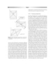
- LEED-Ch-03.qxd 11/27/05 4:22 Page 72 72 Chapter 3 in or at the boundaries of the solid crust, whereas changes in mass due to thermal effects are less common. The fact that forces caused by changes in velocity or acceleration in 200 kg 200 kg space deform the solid crust is witnessed by structures 200 kg formed in the rocky crust by them (Sections 4.14–4.16). 200 kg 3.13.1 Stress A B F = mg Stress, , is forceF, per unit area, A, when acting over a sur- Surface A >> B face (Fig. 3.56). The units for stress are the Pascal (Pa) Fig. 3.57 Stress can be explained as the intensity of force over a which is Newton per square meter (Nm 2). More useful surface. The constant force exerted by the rock ball gives a higher units for the very large stresses relevant to tectonic studies stress when it is put to rest over a column with a smaller surface are the Kilopascal, kPa (103 Pa), Megapascal, MPa area: producing fractures if the internal resistance is exceeded. (109 Pa), and Gigapascal, GPa (1012 Pa). To illustrate the physical difference between force and stress, imagine a ball The resulting stress over the smaller surface is bigger weighing 200 kg. The most important part of solid stress even when the force has the same value in both cases. is the force, the stress itself can be envisaged as the effect In other words, the force is felt with more intensity over or intensity of the force applied to a mass of rock and how the small surface and is thus able to produce deformation it is distributed or felt by the rock in every conceivable easier than over the wide surface. The single vector corre- direction of space. The force exerted by the ball in sponding to the force per unit area which reflects the force Newtons (N) over any surface should be constant: intensity over a surface F/A is called a traction and is only F mg 200 kg · 9.8 ms 2 1,960 N. In a simple one of the infinite components of the overall stress system example, consider the 200 kg ball resting on the top sur- (Fig. 3.58). Because forces can change magnitude or face of a wide column, of area say 2 m2 (Fig. 3.57a). The direction over a surface, we have to define different stress force is distributed over all the surface and the column will values for every infinitesimal part of the surface or at any hold up depending on its material resistance. If the same point as dF/dA. If we consider a surface in a state of equi- force is applied over a surface of a smaller column, for librium, any traction has to be balanced by an equal and example, 0.5 m2, of the same material, the identical force opposite traction. This pair of tractions constitutes the of 1,960 N may lead the column to break (Fig. 3.57b). surface stress (Fig. 3.59b), which can be resolved into nor- Remembering that F/A (Equation 1; Fig. 3.56) the mal and shear components (Fig. 3.59c). It is important to resulting stresses for both columns are 1,960 N/ remember that in a state of equilibrium the sum of the 2 m2 0.98 kPa and 1,960 N/0.5 m2 3.9 kPa, forces acting over a surface equals zero. respectively. We have so far considered only how the stress value is distributed according to a single surface orientated per- pendicular to the applied force. However, the orientation of the surface in relation to the applied force is essential in F (N) determining the resulting traction value and there should ce be an orientation and magnitude for every possible surface For inclined at different angles. The stress tensor is composed A of all the individual surface stresses acting over a given point. Stress analysis can be approached in two dimensions (2D) or three dimensions (3D): in 2D orientations are referred to an xy coordinate system, whereas in 3D an xyz Area (m2) system is used, in which z is conventionally taken as the vertical component. If all the tractions are equal in magni- Stress tude, as occurs in static fluids, the stress tensor has the s = F/A (Nm–2 = Pa) (1) shape of a circle in 2D and of a sphere in 3D; we have seen Stress is force per unit area, measured in Pascals in our discussions of fluid stress (Section 1.16) that such a (Pa) or Nm–2 state is called hydrostatic stress (Fig. 3.58b). In solids, when the tractions usually have different magnitudes, the shape Fig. 3.56 Revision: force and stress.
- LEED-Ch-03.qxd 11/27/05 4:22 Page 73 Forces and dynamics 73 (b) Surface stress –s (a) sn s Surfac e a –s t Su rfa ce (c) sn Surfac –t Traction and traction e (a) Non-Hydrostatic stress tensor components –t z sn Surface stress x components Fig. 3.59 (a) As forces, tractions (forces acting over a surface) can be resolved into a normal ( n) and a shear component ( ); (b) Surface stress, a pair of equal in magnitude and opposed in direction trac- tions at equilibrium; (c) Surface stress components resolved for (b). (b) Hydrostatic stress tensor z x o Fig. 3.58 The stress tensor defines an ellipse in 2D and an ellipsoid in 3D. In the particular case of hydrostatic stress, it defines a circle in y 2D and a sphere in 3D. o of the stress tensor is still very regular but acquires the nature of an ellipse in 2D or an ellipsoid in 3D (Fig. 3.58a). As in fluid forces, solid tractions can be resolved into stress components, one normal to the surface which is called normal traction n and a component parallel to the surface named shear traction, (Fig. 3.59a). It is usual to name these traction components normal stress and shear stress respectively. In the hydrostatic state of stress all trac- tions are normal components and are applied at 90 to all possible surfaces; there are no shear stresses in any direction. In order to have shear stress components, the tractions for different directions have to be unequal and they have to act over a surface orientated at a certain angle different to 90 . Fig. 3.60 Forces acting over a small volume of rock in an outcrop. In order to illustrate this point and to visualize how Many surfaces with different orientations can be defined. We can stresses are distributed in a rock, imagine a mass of sta- extract an imaginary cube and define the tractions acting on the tionary rock in which many different surfaces exist surfaces. (Fig. 3.60). These surfaces are abundant in natural crustal rock and may comprise joints, faults, stratification planes, point, actually over a infinitesimal volume of rock (as points crystal lattices, and so on and even so we can also imagine are dimensionless and lack surfaces) will give the full stress other virtual surfaces which, even when not present at the tensor, with tractions or vectors acting over all the differ- moment, may potentially have been developed or can be ent surfaces with all possible orientations. From the mass developed at some time in the future. Forces acting at a of rock we can extract a tiny imaginary cube over which
CÓ THỂ BẠN MUỐN DOWNLOAD
-

Physical Processes in Earth and Environmental Sciences Phần 1
 34 p |
  71
|
71
|  7
7
-
Physical Processes in Earth and Environmental Sciences Phần 2
0 p | 60
| 6
-
Physical Processes in Earth and Environmental Sciences Phần 6
0 p | 54
| 5
-
Physical Processes in Earth and Environmental Sciences Phần 4
34 p | 46
| 4
-

Physical Processes in Earth and Environmental Sciences Phần 5
34 p | 50
| 4
-
Physical Processes in Earth and Environmental Sciences Phần 8
0 p | 41
| 4
-
Physical Processes in Earth and Environmental Sciences Phần 7
34 p | 45
| 3
-
Physical Processes in Earth and Environmental Sciences Phần 9
34 p | 47
| 3


Chịu trách nhiệm nội dung:
Nguyễn Công Hà - Giám đốc Công ty TNHH TÀI LIỆU TRỰC TUYẾN VI NA
LIÊN HỆ
Địa chỉ: P402, 54A Nơ Trang Long, Phường 14, Q.Bình Thạnh, TP.HCM
Hotline: 093 303 0098
Email: support@tailieu.vn
Giấy phép Mạng Xã Hội số: 670/GP-BTTTT cấp ngày 30/11/2015 Copyright © 2022-2032 TaiLieu.VN. All rights reserved.

