Physical Processes in Earth and Environmental Sciences Phần 9

Chia sẻ: Fwefwefqef Qwdqqfqwf | Ngày: | Loại File: PDF | Số trang:34

Thêm vào BST

Báo xấu

48
lượt xem 3
download

Download Vui lòng tải xuống để xem tài liệu đầy đủ

Chương 6 Các mô hình chính của dòng chảy dốc từ mặt biển tính năng động. Lưu ý sự kiểm soát của các vectơ hiện tại (cả độ lớn và hướng) bởi độ lớn của gradient không gian trong địa hình nước.

Chủ đề:

Bình luận(0) Đăng nhập để gửi bình luận!

Lưu

Nội dung Text: Physical Processes in Earth and Environmental Sciences Phần 9

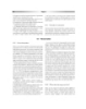
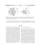
LEED-Ch-06.qxd 11/28/05 10:25 Page 258 258 Chapter 6 LOW LOW 0 0 H HIGH HIGH 0 H H H 0 0 0 LOW LOW LOW +1.3 m –1.1 m 0 HIGH LOW Fig. 6.24 The remarkable satellite-measured topography of the mean sea surface (with wave and tidal wave effects subtracted). LOW GS KS HIGH HIGH HIGH HIGH HIGH HIGH AC AC LOW LOW LOW Fig. 6.25 The major pattern of gradient ﬂow from the computed dynamic sea surface. Note the control of current vectors (both magnitude and direction) by the magnitude of the spatial gradients in water topography, that is, OBL ﬂow is parallel to the gradient lines, with an inten- sity proportional to grayscale thickness. Note western intensiﬁcation of Paciﬁc Kuroshio (KS) and Atlantic Gulf Stream (GS) currents and the strong circumpolar Antarctic current (AC). though complex, meandering ﬁlament of warm Caribbean We have seen that all moving ﬂuid masses possess water in transit to the shores of northwest Europe vorticity appropriate to the latitude in which they ﬁnd (Figs 6.26 and 6.27). In the mid-twentieth century, themselves (Section 3.8) and that the total, or absolute, vor- Stommel explained these most striking features of the ticity (f ) must be conserved. Thus a northward-moving general oceanic circulation by a consideration of both mass of water, impelled by wind shear to spin clockwise, will lateral friction and conservation of angular momentum. gain planetary vorticity as it moves. In order to keep
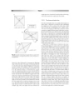
LEED-Ch-06.qxd 11/27/05 2:33 Page 259 Outer Earth processes and systems 259 GS meanders sl cool MAB Mid- sl Atlantic Bight sl water MAB tongue warm sl transports Gulf N and E breach Stream Fig. 6.26 The Gulf Stream is usually a continuous, though complex, meandering ﬁlament of warm Caribbean water in transit to the shores of northwestern Europe. In these satellite images an unusually strong north wind has driven cool waters from the Mid Atlantic Bight across the track of the Gulf Stream, breaching it as a cool tongue that is eventually itself transported north and east in the main current. Main northern margin to Gulf Stream is a boundary shear layer (sl). the northern hemisphere and anticlockwise (to the left) in 80°w 70°w 60°w the southern hemisphere. 45°N 45°N Let us apply these simple notions of conservation of angular momentum to real-world oceanic gyres by a 0 vorticity balance, taking into account the action of wind shear, the change of f with latitude, and the effects of 39°N 39°N boundary layer friction at the ocean edges. The simplest 0 0 physical model for a symmetrical wind-driven gyre would be in 2D and have westerlies and trades blowing opposite 0 33°N 33°N in a clockwise circulation, both declining to zero at the 0 horse latitudes (Fig. 6.28). One can see immediately that 0 the wind velocity gradients will cause a clockwise angular velocity of rotation (i.e. addition of negative vorticity to 27°N 27°N the water) and that the magnitude of the pressure gradi- ents due to Ekman transport will determine the strength 80°w 70°w 60°w of the resulting water ﬂow. We must also take into account 0 the linear rate of change of the planetary vorticity, f, with –50 cm –30 cm –10 +10 +30 +50 cm latitude, as this also determines the transport vector. sea surface height Finally, since we are concerned with solving the problem (1 m of topography over a typical eddy length of c. 250 km gives a mean slope of 1: 250,000: note the asymetric slopes caused by of western intensiﬁcation against the solid boundary of the radial flow around the meandering Stream) continental rise, we recognize that the sense of boundary Fig. 6.27 Map of northwest Atlantic sea surface topography as meas- layer friction will cause the addition of positive vorticity on ured by remote sensing from altimetric satellite Jason-1. The map both western and eastern boundaries. The combined effect shows strong topographic features (mesoscale eddies) associated of wind and f on the western side enhances the negative with meanders of the surface Gulf Stream current. Geostrophic the- vorticity. On eastern margins the two effects roughly cancel ory (Fig. 6.5) says that ﬂow should parallel the topography, deﬁning in this case the sinuous ﬂow around a compex series of warm and out. For the western current to remain steady and in bal- cold core eddies. ance the frictional addition of positive vorticity must be made more intense. This can only be done by increasing the current velocity, since the braking action provided by absolute vorticity constant it must therefore lose relative boundary layer friction is proportional to velocity squared. vorticity. As the major part of the ﬂow away from the ocean The warm western currents are thus extremely strong, up bottom boundary layer is deemed frictionless the external to ten times the strength of the cool eastern currents. ﬂow lags rotation of Earth and therefore loses positive rela- It should not be thought that strong western boundary tive vorticity, that is, gains negative relative vorticity. In currents have no effect at oceanic depths. Direct current other words the ﬂow rotates clockwise (i.e. to the right) in
LEED-Ch-06.qxd 11/27/05 2:33 Page 260 260 Chapter 6 Western half of northern hemisphere circulating gyre Eastern half of northern hemisphere circulating gyre zp ve – zr–ve zr –ve zr –ve zp –ve zp +ve zr –ve zp +ve W-side story: f increases N and so zp more negative N E-side story: f decreases S and so zp more positive S zr from wind stress is negative zr from wind stress is still negative Overall on this westward leg a net decrease of relative Overall on this eastward leg a net balance of relative vorticity (–zp–zr< 0) vorticity (+zp–zr~ 0) Overall, across the whole circuit (west and east combined) there is net loss of vorticity. This is not allowed because the total vorticity must be kept constant. Extra relative vorticity must be generated by either pronounced western lateral boundary shear or by western bottom shear, or a combination of both. The eastern flow needs no such enhancement and is thus weaker and more spatially uniform. West East ζf +ve Fig. 6.28 Sketches to show that conservation of vorticity requires western boundary currents to be stronger than eastern ones. is planetary p vorticity (or f), r is relative vorticity due to wind shear, and f is relative vorticity due to lateral friction. measurements and bottom scour features indicate that Front: this is known to shift zonally by large amounts strong vortex motions are sometimes able to propagate tur- depending upon the amount of cold but buoyant freshwater bulent energy all the way (i.e. 4 km) down to the ocean issuing out of the Arctic from ice melting. ﬂoor, where they cause unsteadiness in the deep thermoha- line current ﬂow (see Section 6.4.5; so-called deep-sea 6.4.4 Internal waves and overturning: storms), enhanced resuspension of bottom sediment, and “Mixing with latitude” nutrient mixing. Also, the currents are unsteady with time, both on the longer time scale, for example, major erosive events on the Blake Plateau have been attributed to Gulf Internal waves (Section 4.10) of much longer period than Stream ﬂow during glacial epochs when the current was normal wind-driven surface waves have recently been dis- thought to be at its strongest, and on a subyearly basis as covered to be a major source of turbulent mixing in the spectacular eddy motions, meanders and cutoffs of cooler deep oceans. The internal wave ﬁeld arises due to wave-like waters form cold-core mesoscale eddies (Figs 6.26 and 6.27). disturbances of the density stratiﬁcation that occurs at var- Notions that the Gulf Stream circulation might “fail” due to ious depths, but particularly within the deep-ocean water global warming and a shutoff in the deep circulation (see column. The disturbances or forcing occurs due to: below) are erroneous: in the words of one oceanographer, 1 Internal tides formed when the main ocean tidal currents “As long as the wind blows and the Earth turns then the ﬂow over rough sea-ﬂoor topography and act upon the inter- surface current will exist.” The one thing that will change is nal stratiﬁcation to form tidal period internal waves. the junction between the warm surface current and the cold 2 A response of the stratiﬁcation to inertial surface waves southerly ﬂows from the Arctic Ocean along the Polar piled up by wind shear during storms, the internal waves
LEED-Ch-06.qxd 11/27/05 2:33 Page 261 Outer Earth processes and systems 261 have periods relating to the Coriolis force and thus are a strong function of increasing latitude. In both cases it is the property of vertical propagation of the internal waves that makes them so effective in spread- ing momentum; unlike surface ocean waves which only propagate horizontally. The internal waves cause vertical internal shear as (du/dz)2 along their wavy interface (cf. Prandtl’s mixing layer theory for turbulent shear ﬂows; Cookie 12) and it is postulated that such shear zones act as in any turbulent boundary layer to transfer turbulent kinetic energy to shorter period eddies as the waves pro- gressively break up. The mixing process is much more Fig. 6.29 The general ocean bottom (darker shading) and surface return legs of the global thermohaline system. Both surface and effective at higher rates of shear and thus the resultant deep currents show periodic breakup into spectacular rotating mixing is more ef ﬁcacious at higher latitudes where the warm-core eddies, shown here for the surface north Brazilian and Coriolis force, f, is greatest. Gulf Stream currents and the deep thermohaline North Atlantic Deepwater in the South Atlantic. 6.4.5 Benthic oceanic boundary layer: Deep ocean currents and circulation We have seen that motion of the upper ocean reﬂects momentum exchange across the atmosphere–ocean S interface as modiﬁed by vorticity gradients from equator S to pole. But what of the deeper ocean? We still know very little of the benthic oceanic boundary layer, as problems of logistics and instrumentation have prevented progress in the area until quite recently. Radioisotope tracers indicate that all deep waters must reestablish contact with the atmosphere on a 500 year timescale. This requires a system of circulation that allows such links. In the last 40 years, theoretical results and detailed temperature, density, and isotopic studies worldwide have revealed a system of deep 17 Sv (1500–4000 m), dense currents (Fig. 6.29), termed ther- mohaline currents from the dual role that temperature and salinity have in producing them. Thus at low latitudes the Fig. 6.30 Cold water sources and generalized ﬂow of North Atlantic upper ocean is heated by solar radiation (density deepwater (T 1.8–4 C). S – major sources of downwelling in the decreases), but also loses water by evaporation (density Labrador and Greeenland seas, the latter due to wind shear by the Irminger tip jet. increases). At high latitudes the upper ocean is cooled by contact with a very cold lower atmosphere during winter (density increases), but freshened by precipitation, river (Fig. 6.30), and by more local shear producing mixing runoff, and inﬂows of polar glacial meltwater (density gyres, as in the mistral wind in the West Mediterranean decreases). At the same time the production of sea ice and the bora of the Adriatic. leads to saltier residual seawater (density increases). Thermohaline currents are linked to compensatory Thermohaline circulation can thus have several causes, intermediate and shallow warmer currents in a compli- most varying seasonally, favored by destabilizing processes cated pattern of downwelling and upwelling, whose that lead to density inversions due to increased surface detailed paths in the Paciﬁc and Indian Oceans are still water density and the production of negative buoyancy. uncertain. The amount of water discharged by the cur- There is also a vital role played in cold water formation by rents is staggering, one estimate for deepwater being some 5 · 107 m3 s 1 (50 Sv [Sverdrup units: each 106 m3 s 1]). atmospheric wind forcing and Ekman suction/pumping (Section 6.2), chieﬂy by regional gyres of high vorticity This is about 50 times the ﬂow of the world’s rivers; about like the Irminger Sea tip jet to the east of Greenland half of the total ocean volume is sourced from the cooled
LEED-Ch-06.qxd 11/28/05 10:29 Page 262 262 Chapter 6 Spain Gibralter gateway Mediterranean m 1,800 2,75 Atlantic 0 m Morocco Fig. 6.31 Deep outﬂow of dense Mediterranean water through the Gibralter gateway. sinking waters of the polar oceans (Fig. 6.30). The nature of the oceanic circulation, with its links from surface to depth, and its role in heat transport and redistribution, has 60 led to its description as a global conveyor belt of both heat and kinetic energy. The consequences of this deep circula- 45 tion are profound, since steady current velocities of up to 0.25 m s 1 have been recorded in some areas where the 30 normally slow (c.0.05 m s 1) thermohaline currents are accelerated on the western sides of oceans (for the same 15 vorticity reasons as discussed earlier for surface currents) >2,000 and in topographic constrictions like gaps between mid- 0 500–2,000 ocean ridges, oceanic fracture zones, and oceanic island 1–500 15 chains and plateaux margins. In all these case turbulent
LEED-Ch-06.qxd 11/27/05 2:34 Page 263 Outer Earth processes and systems 263 zones of the mid-Atlantic Ridge, with intense turbulent polar regions, local erosional resuspension of ocean-ﬂoor mixing along the upper interface. Tracer studies at the muds by “storms” and enhanced thermohaline currents, interface of other shallow water masses reveal a low value windblown dust, and dilute distal turbidity current ﬂows of the mixing rate, about 10 5 m 2 s 1. This implies a low probably all have a role. Some nepheloid layers may be up rate of turbulent mixing along density interfaces relative to to 2 km thick, although 100–200 m is a more usual ﬁgure. lateral spread, a conclusion also established by turbulent Sediment in nepheloid layers is usually 2 m in size stress calculations. However, it is likely that other mixing although ﬁne silt up to 12 m may be suspended, nor- mally at concentrations of up to 500 mg l 1 rising to mechanisms exist, for example breaking internal waves 5000 mg l 1 a few meters off the bottom during deep-sea generated during ocean tides, which will lead to much larger turbulent dissipation. “storms.” Nepheloid layers are also known in many areas A feature of deep ocean waters is attributed in part to from intermediate depths, often at the junction between the action of thermohaline currents and in part to the different water masses. These are thought to arise through occurrence of deep-sea storms (see discussion in the erosion of bottom sediments by internal waves Section 6.4.5). This is the phenomenon of increased sus- (Section 4.13) and tides, ampliﬁed on certain critical bot- pended material, revealed by light-scattering techniques tom slopes. The layers, once formed, intrude laterally into (Fig. 6.32). The source of the suspended sediment in these the adjacent open ocean as layers many tens of meters bottom nepheloid layers is variable: distant sourcing from thick. 6.5 Shallow ocean Shallow ( 200 m depth) ocean dynamics (Fig. 6.33) are bottom and for the longer-period tidal wave to amplify as it more complicated than the open ocean both because of the is forced shelfward from the open ocean. Proximity to land effects of the shallow water on wave and tide and proximity causes interactions of wave and tide with ef ﬂuent plumes to land. A generalized physical description of the shelf sourced from river estuaries and delta distributaries boundary layer (Fig. 6.34) deﬁnes an inner shelf mixed (Fig. 6.35). Coastal geometry also has a strong local inﬂu- layer where frictional effects of wave and tide are dominant ence upon water dynamics. Shelves have been classiﬁed into in the less than 60 m shallow waters. In the deepening tide- and weather-dominated, but most shelves show a mid- to outer shelf there is differentiation into surface and mixture of processes over both time and space. The major- bottom boundary layers separated by a “core” zone. The ity of shelves have a tidal range less than 2 m but this may shallow water enables waves to directly inﬂuence the be ampliﬁed several times around their margins. Intruding ocean Tidal Meteorological Density currents currents currents currents reversing, standing waves or rotary boundary (Kelvin) waves Cyclic Residual Longshore Direct wind components components and rip currents shear Wind Wind drift setup Landward Shelf Shelf Internal bottom riverine riverine waves currents jets and plumes underflows Fig. 6.33 Components of the shelf current velocity ﬁeld.
LEED-Ch-06.qxd 11/27/05 2:34 Page 264 264 Chapter 6 6.5.1 Shelf tides Tidal strength may also vary because of the nature of the connection between the shelf or sea and the open ocean. In the case of the Mediterranean Sea, for example, the In the oceans the twice-daily tidal wavelength, , is very connection with the Atlantic has become so narrow and large (about 104 km) compared with water depth, h (say restricted that the Atlantic tide cannot reach any signiﬁ- 5 km), and is thus still of shallow-water (long-wave) type cant range over most of its area. Locally, in the Straits of (i.e. h/ 0.1). From Section 4.9 the maximum tidal Gibraltar, the Straits of Messina, and the Venetian Adriatic, wave velocity in the open oceans is thus given approxi- for example, the tidal currents (but not necessarily the tidal mately by u (gh)0.5, about 220 m s 1. The open ocean range) may be greatly ampliﬁed when water levels between tidal wave decelerates as it crosses the shallowing waters of unrelated tidal gyres or standing waves interrelate. the shelf edge. This causes wave refraction of obliquely Another cause of spatially varying tidal strength is the incident waves into parallelism with the shelf break and resonant effect (Section 4.9) of the shelf acting upon the partial reﬂection of normally incident waves. At the same open oceanic tide (Fig. 6.36) and creating standing waves. time the wave amplitude, a, of the transmitted tidal Resonance greatly increases the oceanic tidal range in wave is enhanced. This follows from the energy equation nearshore environments and leads to the establishment of for gravity waves E 0.5 ga2(gh)0.5 (Section 4.9); the very strong tidal currents. Most shelves are too narrow and supremacy of the square versus the square root terms deep (Fig. 6.36) to show signiﬁcant resonance across means that the overall wave amplitude must increase. The them, that is, L 0.25 . In most cases, for example in the tidal current velocity of a water particle (as distinct from shelf of the eastern USA, a simple slow linear increase of the tidal wavelength) also increases because this depends tidal amplitude and currents occurs across the shelf. Open upon the instantaneous amplitude of the wave. coastal basins like estuaries, bays, and lagoons must receive the 12-hourly oceanic tidal wave and a standing wave (of Shoreface Inner shelf Mid shelf Outer shelf period 12 h) may be set up, with a node at the mouth and an antinode at the end (by no means the only resonant possibility). In the limiting scenario, with L 0.25 , we Surface boundary layer Mixed b.l. have T 4L/ gh . The Bay of Fundy, Maritime Canada, Benthic b. l. is the world’s most spectacular example of a gulf that res- onates with the c.12 h period of the semidiurnal ocean tide. The gulf has a length of about 270 km (calculated from the gulf head to the major change of slope at the Fig. 6.34 Simple division of shelf waters into mixed, surface, and shelf edge) and is about 70 m deep on average, giving bottom boundary layers. Inner shelf mixed b.l. has tide and wave the required approximately 12 h characteristic resonant mixing, though the degree of mixing is seasonally variable. Outer period. The standing resonant oscillation has a node at its shelf is often stratiﬁed into a surface b.l. with geostrophic ﬂows and entrance, which causes the tidal range to increase from a friction-dominated benthic boundary layer. Riverine estuary Wind shear and drift currents or delta distibutary 40–80 m water depth es g ce tin av hfa ota ew c d r aves Bea Buoyant ac n ls ga lw cel Surf plume sin ida Rip ver vin) t Re el (K s ave Seasonal thermocline Se mw tup r sto gra Internal waves by die ion nt c s Ero u rren ts Fig. 6.35 Major controls on cross-shelf water and sediment transport.
LEED-Ch-06.qxd 11/28/05 10:38 Page 265 Outer Earth processes and systems 265 6 Plan Plan Shelf depths Relative tidal wave amplitude 100 m 4 50 m 25 m 2 Flood tide Ebb tide t=0 t = 6/12T Pressure force Pressure force 0 0.5 1.0 1.5 0 Shelf width in tidal wavelengths x-section x-section Fig. 6.36 Tidal wave resonance across shelves of different width and Coriolis force Coriolis force water depth. 3 m to a spring maximum of some 15.6 m along its length Cotidal lines and amphidromic point to the antinode. 3 4 2 The Coriolis force acts as a moderating inﬂuence on tidal streams in semi-enclosed large shelves, like the north- 5 1 western European shelf, the Yellow Sea, and the Gulf of 6 Ap 0 St. Lawrence. In the former, the progressive anticlockwise 7 11 tidal wave of the North Atlantic enters ﬁrst into the Irish Sea and the English Channel and then several hours later it 8 10 veers down into the North Sea proper through the Norway–Shetland gap in a great anticlockwise rotary wave (whose passage north to south was noted by the monk Bede in the eighth century). Why should such rotary motions occur? The answer is that the tidal gravity wave, unlike normal surface gravity waves due to wind shear or t=9 swell (Section 4.9), has a sufﬁciently long period that it Times in 1/n of 12 h tidal period must be deﬂected by the Coriolis force. Since the water on continental shelf embayments like the North Sea is Fig. 6.37 The development of amphidromic circulation within a partly enclosed shelf sea by Coriolis turning of the tidal wave into bounded by solid coastlines, often on two or three sides, a Kelvin wave of circulation. the deﬂected tide rotates against the sides (Figs 6.37 and 6.38) as a boundary wave. Such waves of rotation against solid boundaries are termed Kelvin waves, the propagating radius of the roughly circular basin and is also a cotidal line wave being forced against the solid boundaries by the along which tidal minima and maxima coincide. effects of the Coriolis parameter, f. The water builds up as Concentric circles drawn about the node are lines of equal a wave whose radial slope exerts a pressure gradient that tidal displacement. Tidal range is thus increased outward exactly balances the Coriolis effect at equilibrium from the amphidromic node by the rotary action. Further (Fig. 6.39). Tidal currents due to the wave are coast paral- resonant and funnelling ampliﬁcation may of course take lel at the coast (Fig. 6.40a) with velocities at maximum in place at the coastline, particularly in estuaries (see the crest or trough (reverse) and minimum at the half- Section 6.6.3). Not all basins can develop a rotary tidal wave height. The wave decays in height exponentially sea- wave: there must be sufﬁcient width, since the wave decays ward toward an amphidromic node of zero displacement. away exponentially with distance. The critical width is The resonant period in the North Sea is around 40 h, a termed the Rossby radius of deformation, R, given by the ﬁgure large enough to support three multinodal standing ratio of the velocity of a shallow-water wave to the magni- waves (Fig. 6.41). The crest of the tidal Kelvin wave is a gh/f . At tude of the Coriolis parameter, that is, R
LEED-Ch-06.qxd 11/27/05 2:34 Page 266 266 Chapter 6 Ap Fig. 6.38 The Kelvin rotating tidal wave travels anticlockwise in the northern hemisphere, decreasing in amplitude inward toward the ampho- dromic point, Ap, of zero displacement. Force balance and Rossby radius of deformation (L). Horizontal pressure gradient force Coriolis force L Fig. 6.39 Topography and bottom ﬂow associated with the edge of an anticlockwise-rotating Kelvin tidal wave. The rotary component is neglected for clarity. this distance the amplitude of any Kelvin wave has reduced (Fig. 6.40). For example, the inequality between ebb and to 1/e, 0.37 of its initial value. ﬂow on the northwest European continental shelf is largely We may usefully summarize the vector variation of tidal determined by a harmonic of the main lunar tide. Since sed- currents by means of tidal current ellipses whose ellipticity is iment transport is a cubic function of current velocity it can a direct function of tidal current type and vector asymmetry be appreciated that quite small residual tidal currents can
LEED-Ch-06.qxd 11/27/05 2:34 Page 267 Outer Earth processes and systems 267 (a) (b) (c) 3, 4 HW +1 2, 5 1, 6 +3 +11 +5 +9 +7 7, 12 8, 11 9, 10 Fig. 6.40 Tidal current variations with time. (a) Linear symmetrical ebb-ﬂood with zero residual; (b) symmetrical tidal ellipse with zero resid- ual current; (c) Irregular tidal ellipse with complex residuals. cause appreciable net sediment transport in the direction of tidal currents ( 0.3 m s 1). Also it is not uncommon for the residual current. The turbulent stresses of the residual the inner shelf to shoreface to be tide-dominated during currents will be further enhanced should there be a superim- the summer months but wave-dominated during the posed wave oscillatory ﬂow close to the bed (Section 4.10). winter. In any case, tidal currents and wave currents are A further consideration arises from the fact that turbulence progressively less important offshore, so that at the outer intensities are higher during decelerating tidal ﬂow than dur- shelf margin it is only the largest storms that affect the ing accelerating tidal ﬂow, due to unfavorable pressure gra- bottom boundary layer. In these areas it is common to dients. Increased bed shear stress during deceleration thus find a multilayer water system, with a surface boundary causes increased sediment transport compared to that during layer dominated by wind shear effects, a middle “core” acceleration, so that the net transport direction of sediment layer, and a basal boundary layer dominated by will lie at an angle to the long axis of the tidal ellipse. upwelling, downwelling, or intruding ocean currents A ﬁnal point concerns the importance of internal tides (Fig. 6.34). Winter wind systems assume an overriding and other internal waves (Section 4.9), particularly in the dominance on most shelves, causing net residual currents outer shelf region. These are common in summer months arising from wind drift, wind set-up, and storm surge. when the outer-shelf water body is at its most density- Wind shear causes water and sediment mass transport at stratiﬁed, with a stable warm surface layer of thickness h an angle to the dominant wind direction because of and density 1 overlying a denser layer, 2. They are also the Ekman effect arising from the influence of the common in fjords. If a wave motion is set up at the stable Coriolis force (see Section 6.2). For example, southward- density interface (due to storm-induced wind stress or the blowing, coast-parallel winds with the coast to the left incoming tide), the restoring force of reduced gravity, is in the northern hemisphere will cause net offshore much smaller than at the surface and so the internal waves transport of surface waters and the occurrence of cannot be damped quickly; they provide important mixing compensatory upwelling. mechanisms when they break at external boundaries. From all this the reader can appreciate that outer-shelf dynamics are extremely sensitive to the magnitude of shelf 6.5.2 Wind drift shelf currents wind systems. Depending upon dominant wind regime, either import or export is possible: for example, cool shelf Although all continental shelves suffer the action of waters can be driven far oceanward as intruding tongues storms, weather-dominated shelves are those that also that may interfere with ocean currents like the Gulf Stream show low tidal ranges ( 1 m) and correspondingly weak (Section 6.4).
LEED-Ch-06.qxd 11/27/05 2:34 Page 268 268 Chapter 6 10 8 9 10 7 1.5 1 11 6 3 2 12 Ap 3 0 3 0.5 1 2 2 3 1 Ap 4 4 5 10 5 6 7 11 6 7 Ap 7 1 5 12 3 10 4 4 5 5 6 Fig. 6.41 Amphidromic tidal gyres of the North Sea and surrounding areas. Each of the the three systems has anticlockwise sense of rota- tion. Full lines are co-range lines with tidal range in meters. Dotted lines are cotidal lines indicating the level of high water at the stated number of hours lapsed since the Moon passed over the Greenwich meridian. 6.5.3 Storm set-up and wind-forced geostrophic London), in the Bay of Bengal, and in the Venetian currents Adriatic (where in both places the inhabitants are not so lucky). The very low barometric pressures during storms cause a sea-level rise under the storm pressure minimum. Let us examine the effects of storm winds in more detail, The magnitude of this effect is about 1 cm rise per mil- for, as we shall see later, major shelf erosion and deposi- libar decrease of pressure. So passage of the eye of a trop- tion result during such episodes. As in lakes, wind shear ical storm of pressure 960 mbar might cause a few tens of drift causes set-up of coastal waters; should this coincide centimeters of sea-level rise. The very low core pressures of with a spring high tide, then major coastal ﬂooding coastal tornadoes are particularly effective at raising the results. The effects are well known in the southern North setup of shelf waters, sometimes up to 4 m or more above Sea (where the Thames Barrage now protects low-lying
LEED-Ch-06.qxd 11/27/05 2:34 Page 269 Outer Earth processes and systems 269 mean high-water level, as in Hurricane Carla on Padre nature of storm surges enables prediction for vulnerable Island, Gulf of Mexico. areas like the North Sea and the Adriatic by reference to The magnitude of wind shear setup can be roughly esti- monitored upcurrent changes in sea level during storm mated by assuming that the shearing stress, , due to the development. Offshore, the large wave setup during wind balances the pressure gradient due to the sloping sea storms means that a compensatory bottom ﬂow occurs out surface, p/ x, that is gh p/ x, where h is water to sea, driven by the onshore to offshore pressure gradient. depth and is water density. Solving for the slope term for Such geostrophic or gradient currents (which are also storm winds of 30 m s 1 acting on 40 m water depth yields turned by Coriolis forcing; Fig. 6.42) have been proven about 2.2 10 6 for the 600 km long North Sea, leading to by measurements during storms to reach over 1 m s 1, a superelevation of about 1.3 m. This is 50 percent or so running for several hours (a fact suspected by submariners less than the observed surge height because we have neg- since 1914, see Fig. 6.42). They are a major means of off- lected important effects due to the Coriolis force, which shore transport from coast to shelf. pushes the current against adjacent shorelines where it is further ampliﬁed by resonance and funneling. In the case 6.5.4 Shelf density currents of the major southern North Sea storm of 1953, the southerly directed wind drift was ﬁrst forced westward onto the Scottish coast with the southward traveling Density currents are also important in shelf transport. (anticlockwise) Kelvin tidal wave, where it ultimately gave Hypopycnal (positively buoyant) jets of fresh to brackish rise, some 18 h later to a 3.0 m superelevated surge water with some suspended sediment issue from most along the Dutch and Belgian coasts. The Kelvin wave estuaries and delta distributary mouths. In higher (c) (a) Storm wind Mid-depth geostrophic Setup flow MSL Gradient Oscillatory current boundary Bottom layer flow Bottom flow (b) Coriolis force Force balance and uniform steady flow Resultant Pressure force force Friction force The earliest recorded direct impression of storm waves (and Coriolis ?gradient currents) from the sea bottom occurs in the log of force HM submarine, E10, in 1914 in the southern North Sea, off Heligoland. After torpedoing a German cruiser the sub bottomed to 30 m and thereafter a very bad storm grounded Pressure and shifted her despite over 10 tons of negative buoyancy gradient force Fig. 6.42 Shoreface to shelf geostrophic gradient currents. (a) Section; (b) force balance; (c) plan.
LEED-Ch-06.qxd 11/28/05 3:20 Page 270 270 Chapter 6 latitudes, small to moderate buoyancy fluxes are soon mid-shelf or right across the shelf break, depending upon turned by the Coriolis force, and they may be trapped their dynamic characteristics and those of the shelf. Low along-source in the mid- to inner shelf where they form slopes encourage long passage, whilst the development of coastal currents or linear fronts. Mixing vortices develop vorticity on steeper slopes encourages turning and termi- along the free shear layer of the fronts and offshore cir- nation. The large buoyancy flux of many late spring and culating shelf waters. Plumes are very sensitive to the summer Arctic rivers, for example, causes plumes to effects of coastal upwelling or downwelling currents extend for up to 500 km offshore, well into the Arctic caused by winds. They may reach some way out into the Ocean. 6.6 Ocean–land interface: coasts Coasts are dynamic interfaces between land and sea where a wide surf zone in which the waves steepen slowly, show energy is continuously being transferred by the action of low orbital velocities, and surge up the beach with very traveling waves, including the tide. This incoming wave minor backwash effects. energy ﬂux also interacts with energy inputs from the land, The shallow water nature of incoming coastal waves in the form of river ﬂows. The nature of any coastal inter- means that the wave trains are no longer made up of dis- face varies according to the type and magnitude of these persive waveforms, as for deepwater waves (Section 4.9). various energy ﬂuxes and also to the geological situation Instead, the speed depends only upon water depth and so determined by bedrock type (more or less resistant). Like the impact of waves upon shallow topography leads to a any interface the coast may be largely static in time and number of interesting features, chieﬂy the familiar curva- space or it may be highly mobile, either advancing seaward ture or refraction of approaching oblique wave crests as when sedimentary deposition dominates, a prograding they “feel bottom” at different times (Fig. 6.45). coastline, or retreating landward when erosion and net transport outward to the shelf dominates, a retreating 6.6.2 Waves arriving at coasts: The role of coastline. radiation stress 6.6.1 Nearshore wave behavior The forward energy ﬂux or power associated with waves approaching a shoreline (Section 4.9) is, Ecn, where E is As the typical sinusoidal swell of the deep ocean passes the wave energy per unit area, c is the local wave velocity, landward over the continental shelf the dispersive wave and n 0.5 in deepwater and 1 in shallow water. Because groups (Section 4.9) undergo a transformation as they of this forward energy ﬂux there exists a shoreward- react to the bottom at values of between about 0.5 and directed momentum ﬂux or radiation stress outside the 0.25 of wavelength, . In this transformation to shallow- zone of breaking waves. This radiation stress is the excess water waves, wave speed and wavelength decrease whilst shoreward ﬂux of momentum due to the presence of wave height, H, increases. Peaked crests and ﬂat troughs groups of water waves, the waves outside the breaker zone develop as the waves become more solitary in behavior exerting a thrust on the water inside the breaker zone. until oversteepening causes wave breakage. Waves break This thrust arises because the forward velocity associated when the water velocity at the crest is equal to the wave with the arrival of groups of shallow-water waves gives rise speed. This occurs as the apical angle of the wave reaches a to a net ﬂux of wave momentum (Fig. 6.46). For wave value of about 120 . In deepwater the tendency toward crests advancing toward a beach there are two relevant breaking may be expressed in terms of a limiting wave components of the stress, ij. One is xx, with the x-axis in steepness given by H/ 0.14. Breaking waves spill, the direction of wave advance and the other, yy, with the plunge, or surge (Figs 6.43 and 6.44); the behavior varies y-axis parallel to the wave crest. These components are according to steepness of the beach face. Steep beaches E/2 for deepwater or 3E/2 for shallow water, and xx possess a narrow surf zone in which the waves steepen rap- 0 for deepwater or E/2 for shallow water. Radiation yy idly and show high orbital velocities. Wave collapse is stress plays an important role in the origin of a number of dominated by the plunging mechanism and there is much coastal processes, including wave setup and setdown, interaction on the breaking waves by backwash from a pre- generation of longshore currents, and the origin of rip vious wave-collapse cycle. Gently sloping beaches show currents (Fig. 6.47).
LEED-Ch-06.qxd 11/27/05 2:34 Page 271 Outer Earth processes and systems 271 The nearshore current system may include a remarkable cellular system of circulation comprising rip currents. The narrow zones of rip currents make up the powerful “undertow” on many steep beaches and are potentially hazardous to swimmers because of their high velocities Swell waves (several meters per second). Rip currents arise because of E1c1 variations in wave setup along steep beaches. Wave setup is Breaking wave the small (centimeter to meter) rise of mean water level above still water level caused by the presence of shallow- water waves. It originates from that portion of the Spilling waves steepen and then collapse Amplifying waves Plunging waves steepen , curl over, and impact E2c2 ash e wave sw ergy of th Kinetic en Surging waves steepen and surge as a bore Energy flux of swell wave = Energy flux of shoreface wave or E1c1 = E2c2 Fig. 6.43 A familiar sight on the sea or lake coast; swell waves slow- ing down (c1 c2) and amplifying over the shelving coast, increasing in height and steepness until they break on the beachface. Energy Fig. 6.44 Types of breaking waves. ﬂux (power) is conserved throughout until ﬁnally dissipated in the turbulence, cavitation, and sediment transport of the swash zone. c2 Ray 1 Ray 1 Ray 2 Ray 2 Shallower E2 s2 h3 Crest u2 h3 Isobath h2 h2 h1 u1 h1 DEEPER slower c1 Kinematic/geometric relations sin u1 c1 gh1 h1 h1 s1 = = = = Crests swing into sin u2 c2 h2 gh2 h2 parallelism with Rays are the bathymetric E1 drawn normal Energy conservation relations Faster contours to wave crests E1 s1= E2s2 H12 s1 = H22 s2 Fig. 6.45 Wave refraction from deeper to shallower water by shallow water waves of height H whose speed is purely a function of water depth.
LEED-Ch-06.qxd 11/27/05 2:34 Page 272 272 Chapter 6 rip cells also exist on long straight beaches with little Sign convention variation in offshore topography, another mechanism must +z, w Plane surface +y,v also act to provide lateral variations in wave height. This is parallel to y thought to be that of standing edge waves (Fig. 6.48), tyy normal to x which form as trapped waveforms due to refraction and +x,u refracting wave interactions with strong backﬂowing wave Wave crests normal txx swash on relatively steep beaches. Edge waves were ﬁrst to plane (shore) c detected on natural beaches as short-period waves acting a x at the ﬁrst subharmonic of the incident wave frequency, w u decaying rapidly in amplitude offshore. The addition of Wave group energy h r = Water incoming waves to edge waves give marked longshore vari- e.g. flux of per unit area density x-momentum ations in breaker height, the summed height being great- E = 0.5rga2 per unit vol. is est where the two wave systems are in phase. It is thought (ru)u = txx that trapped edge waves may be connected with the for- bottom mation of the common cuspate form of many beaches; Fig. 6.46 Deﬁnition diagram for the radiation stress, , exerted on these have wavelengths of a few to tens of meters, approx- the positive side of the xy plane by wave groups approaching from imately equal to the known wavelengths of measured edge the left hand side. The radiation stress is the momentum ﬂux waves. Results concerning the effects of edge waves and (i.e. pressure) due to the waves. “leaky” mode standing waves (where some proportion of energy is reﬂected seaward as long waves at infragravity frequency, 0.03–0.003 Hz) indicate that both shoreward and seaward transport may result, dependent on 30 conditions. Usually, water entrained under groups of large waves in arriving wavepackets is preferentially transported Mean water level (mm) seaward under the trough of the bound long period 20 group wave. p Beach ram Setup The familiar longshore currents are produced by oblique wave attack upon the shoreline; these may be 10 superimposed upon the rip cells described earlier. Such currents, which give a lateral thrust in the surf zone, are Still water level caused by xy, the ﬂux toward the shoreline (x-direction) of 0 momentum directed parallel to the shoreline (y-direction). –5 Theory Experiment This is given by xy 0.25E sin 2 , where is the angle Setdown between wave crest and shore (shore-parallel crests 0 ; Fig. 6.47 Wave setup and setdown as produced by radiation stress shore-normal 90 ). The xy value reaches a maximum caused by incoming waves in an experimental tank. when sin 2 1, or when the angle of wave incidence is 45 . Field data give the longshore velocity component, ul, as 2.7umax sin cos . radiation stress xx remaining after wave reﬂection and bottom drag and is balanced close inshore by a pressure 6.6.3 Estuarine circulation dynamics gradient due to the sloping water surface (Fig. 6.48). In the breaker zone the setup is greater shoreward of large Water and sediment dynamics in estuaries are closely breaking waves than smaller waves, so that a longshore dependent upon the relative magnitude of tide, river, and pressure gradient causes longshore currents to move from wave processes. The incoming progressive tidal wave is areas of high to low breaking waves. These currents turn modiﬁed as it travels along a funnel-shaped estuary whose seaward where setup is lowest and where adjacent currents width and depth steadily decrease upstream. For a 2D converge. wave that suffers little energy loss due to friction or reﬂec- What mechanism(s) can produce variations in wave tion (a severe simpliﬁcation), the wave energy ﬂux will height parallel to the shore in the breaker zone? Wave remain constant, causing the wave to amplify and shorten refraction is one mechanism; some rip current cells are as it passes upstream into narrower reaches. This is the closely related to offshore variations in topography. Since
LEED-Ch-06.qxd 11/27/05 2:34 Page 273 Outer Earth processes and systems 273 Uniform incoming waves Small Small Large Node Node node breakers breakers breakers Momentum flux Momentum flux Antinode out out reinforcement of edge wave crests Momentum Flux Rip Cell Rip Cell in Longshore currents Large setup Swash Swash Edge wave Edge wave ray crests reinforced Beach Beach Fig. 6.48 Rip current cells located in areas of small breakers where incoming waves and standing edge waves are out of phase. convergence effect. Thus for wave energy, E, per unit length circulatory advection. Viewed in this way, water dynamics of an estuary, Eb is the energy per unit length, where b is in estuaries may be conveniently represented by four major total estuary width. Multiplying by the wave speed, c, gives end-members (Fig. 6.49). However, it is important to the energy ﬂux up the estuary as Ebc constant. Writing realize that a single estuary may change its hydrodynamic E ( ga2)/2 and the wave equation for shallow water character with time according to changing river, tidal, and waves as c (gh)0.5, we have 0.5( ga2)b gh 5 constant, wave conditions. or, a ∝ b 0.5h 0.25. We can see that narrowing has more Type A well-stratiﬁed estuaries are those river-dominated effect on changing wave amplitude than shallowing. estuaries where tidal and wave mixing processes are Shallowing also causes the wave speed to decrease and, permanently or temporarily at a minimum. The stratiﬁed since wave frequency is constant, the wavelength must system is dominated by river discharge, with the decrease by the argument c f . Since c/f gh/f , tidal : river discharge ratio being low, less than 20. An we have ∝ h0.5. Thus tidal waves increase in amplitude upstream tapering salt wedge occurs, over which the fresh and decrease in wavelength up many estuaries. But we can- river water ﬂows as a buoyant plume (Fig. 6.50). Shear not ignore frictional retardation of the tidal wave in this waves of Kelvin–Helmholtz type may occur at the halocline discussion; this causes a reduction in amplitude of the tide interface, the waves cause upward advective mixing of salt upstream and is greatest when channel depth decreases water with fresh water. Should ﬂow occur over topography rapidly. In some estuaries the tidal wave changes little in then internal solitary wave trains may be triggered at the amplitude since the convergence effect is balanced by interface. A prominent zone of deposition and shoaling at frictional retardation. Resonant effects with tide or wave the tip of the salt wedge arises when sediment deposition may also affect currents in estuaries (Section 6.6). from bedload occurs in both fresh water and seawater. This The most fundamental way of considering estuarine zone of deposition shifts upstream and downstream in dynamics is through the principle of mass conservation, response to changes in river discharge and, to a much which states that the time rate of change of salinity or sus- lesser extent, to tidal oscillation. pended sediment concentration at a ﬁxed point is caused Type B partially stratiﬁed estuaries are those in which tur- by two contrasting processes: turbulent diffusion and bulence destroys the upper salt–wedge interface, producing
LEED-Ch-06.qxd 11/27/05 2:34 Page 274 274 Chapter 6 a more gradual salinity gradient from bed to surface water turbidity maximum is also acted on by gravity-induced by intense turbulent mixing. The tidal : river discharge circulations arising from excess density. ratio is between about 20 and 200. Down-estuary changes Type C well-mixed estuaries are those in which strong in the salinity gradient at the mixing zone occur so that the tidal currents completely destroy the salt-wedge/fresh- zone moves upward toward higher salinities. Earth rota- water interface over the entire estuarine cross-section. The tional effects cause the mixing surface to be slightly tilted ratio of tide : river discharge is greater than 200. so that in the northern hemisphere the tidal ﬂow up the Longitudinal and lateral advection processes dominate. estuary is nearer the surface and strongest to the right. Vertical salinity gradients no longer exist but there is a Sediment dynamics is strongly inﬂuenced by the upstream steady downstream increase in overall salinity. In addition, and downstream movement of salt water over the various the rotational effect of the Earth may still cause a pro- phases of the tidal cycle. The resulting turbidity maximum nounced lateral salinity gradient, as in Type B estuaries. is particularly prominent in the upper estuary (around Transport dynamics are dominated by strong tidal ﬂow, 1–5 ppt salinity) on spring and large neap ebb and ﬂood with estuarine circulation gyres produced by the lateral tidal phases, and less prominent at slackwater periods due salinity gradient. Extremely high suspended sediment con- to settling and deposition. Turbidity maxima are affected centrations may occur close to the bed in the inner reaches by the magnitude of freshwater runoff. A seasonal cycle of of some tidally dominated estuaries. Sediment particles of dry-season upstream migration of the turbidity maximum river origin, some ﬂocculated, will undergo various trans- and locus of maximum deposition is followed by wet-season port paths, usually of a “closed loop” kind (Fig. 6.51), in downstream migration and resuspension by erosion. The response to settling into the salt layer and subsequent 3D Salinity gradients Freshwater buoyant River flow River flow Mixing around plume internal waves g Intense turbulent mixin salt wedge Type A: well-stratified estuary Type B: partially stratified estuary 2D Salinity gradients in horizontal River flow Negligible river flow Near-homogenous salinity g Intense turbulent mixin Type C: well-mixed estuary Type D: completely mixed estuary Fig. 6.49 A useful classiﬁcation of estuaries according to the dynamic processes of mixing and salinity gradients. sed. conc. (mg l–1) Flow velocity (m s–1) 10 5 Salinity (‰) 0 0 5 30 20 2 10 15 Mixin River 4 g 20 Water Zone 25 Depth m 40 6 8 Salt Wedge 10 10 50 12 High-sediment Estuary bed Estuary concentration mouth gradients 5 km Fig. 6.50 Salinity, velocity, and suspended sediment proﬁles taken during high tide along transect of the well-stratiﬁed (salt wedge) Fraser River estuary.
LEED-Ch-06.qxd 11/27/05 2:35 Page 275 Outer Earth processes and systems 275 0 0.6 Sediment Mean streamwise concentration velocity Flood tide Ebb tide Depth below flow surface Concentration, kg m–3 Turbulent shear flow 0.3 Deposition Settling Resuspension Advection Deposition Mobile turbulent suspension Resuspension 0.0 –0.8 0.0 0.8 Mean flow velocity, m s–1 Lutocline Fig. 6.51 Variation of estuarine suspended sediment concentration Mobile fluid mud Bingham Plastic Flow over several tidal cycles. Velocities are negative for the ﬂood (incom- ing) tide and positive for the ebb. Stationary fluid mud Cohesive sedimented bed 0 Sediment concentration or flow velocity transport by the net upstream tidal ﬂow. Settling of bound Fig. 6.52 To illustrate the process of ﬂuid mud formation. aggregates of silt- and sand-sized particles creates large areas of stationary and moving mud suspensions (Figs 6.52 and 6.53), loosely termed ﬂuid mud, that char- Concentration 2 acterize the outer estuarine reaches of tide-dominant estu- profiles aries. This may be mobile or ﬁxed, the latter grading into after 1 hour areas of more-or-less settled mud. Stationary suspensions Initial conc. Initial conc. 1.5 1 g l –1 5.5 g l –1 up to 3 m thick can show sharp upper surfaces on sonar records and may deposit very quickly. Such suspensions Elevation, m form during slackwater periods, progressively thickening 1 during the spring to neap transition. They are easily Concentrated Dilute eroded, to be taken up in suspension once more by the suspension suspension accelerating phases of spring tidal cycles. Type D estuaries are theoretical end-members of the 0.5 estuarine continuum in that they show both lateral and Lutocline vertical homogeneity of salinity. Such conditions apply only in the outer parts of many type B and C estuaries; 0 0.1 1 10 they are clearly transitional to open shelf conditions. Concentration, g l –1 Under equilibrium conditions, saline water is diffused Fig. 6.53 Experimental data to contrast the behavior of dilute and upstream to replace that lost by advective mixing. concentrated settling sediment suspensions. Note the stepped proﬁle Sediment movement is dominated entirely by tidal that forms in the latter case with the formation of a lutocline as hin- motions, again with no internal sediment trap. dered settling and ﬂocculation delay fall. between closely located clay particles is made positive by 6.6.4 Estuarine sedimentation absorption of abundant cations from salt water. Also, the higher the amount of suspended clay, the more likely particle collisions will occur, leading to ﬂocculation of The mixing of fresh and salt water causes estuarine circu- aggregates whose settling velocity is enhanced. At the lation in response to density gradients. Sedimentary parti- same time, the higher the particle concentration, the cles may be of both marine and river origin, with lower will be the rate of settling as a result of the effects of ﬂocculation and ﬂoc destruction by turbulent shear and particle hindrance (Section 4.7). These two effects, resuspension of bed material as important controls upon agglomeration and hindrance, lead to the formation of particle size. Flocculation is a process whereby the usually distinct layers of suspended material during the period of repulsive van der Waals electrostatic forces present
LEED-Ch-06.qxd 11/27/05 2:35 Page 276 276 Chapter 6 relatively slack water in estuaries where tidal currents are delta distributary (Fig. 6.54). This occurs as a jet, analogous important (Figs 6.52 and 6.53). The net accumulation of to the expanding ﬂow of ﬂuid issuing from any nozzle or sediment in the water column due to tidal pumping arises opening (Section 4.1). The nature of the discharge, the because of inequality in the local magnitude of the physiography of the receiving basin, and the degree to ebb and ﬂood tides. If the ﬂood is dominant in the upper which the discharge is modiﬁed by wave and tide will con- estuary, as is often the case, then more sediment enters trol the gross morphology of a delta and the distribution the upper estuary than leaves, and hence a turbidity of sediment. Bates ﬁrst considered the role of jets as rele- maximum occurs. vant and essential to the theory of delta formation. As ef ﬂuent ﬂuid moves into the marine basin it has the possi- bility to expand in both horizontal and vertical directions. 6.6.5 Delta distributaries Plane jets just expand horizontally while axial jets expand in all directions. Gently sloping coasts restrict vertical Consider the nature of the combined discharge of sedi- expansion and cause plane jet formation. Buoyant effects ment and fresh water issuing from the mouth of a major between ef ﬂuent and ambient ﬂuids can give rise to re New Orleans Frictional jet (homopycnal) Gentle offshore Abandoned gradient St Bernard delta Typical of shoal water interdistributary bays Typical of major distributary outlets Abandoned re Mixing Laforche delta ra Positively buoyant plume Salt wedge (hypopycnal) Fig.6. 54 Coastal jets illustrated from the Mississippi “birdsfoot” delta. Efﬂuent jets and plumes rich in suspended sediment appear gray in this satellite image. Note the form of this river-dominated delta, with its numerous distributaries issuing from the seaward extension of the main river channel. The pattern of these gives rise to the term “birds-foot” delta. Most sediment deposition occurs during high river ﬂow close to the mouths of the distributaries, forming accumulations of sediment called “mouth bars.” Note the abandoned older Holocene deltas to the southwest and northeast, which are now being reworked by wave action under conditions of rising local relative and absolute sea level: the city of New Orleans is immensely vulnerable to both river ﬂooding and marine inundation during major hurricane impact, as events of summer 2005 have proved.
LEED-Ch-06.qxd 11/27/05 2:35 Page 277 Outer Earth processes and systems 277 signiﬁcant gravitational body forces of the form re [( a e)/ a] g per unit volume of ef ﬂuent ﬂuid, where a is ambient density and e is ef ﬂuent ﬂuid density. The Mix ing behavior of the plume thus depends upon the resultant of Inertial jet (homopycnal) the various buoyancy contributions due to temperature, ra salinity, and suspended sediment concentration. For example, negative buoyancy acts when sediment-laden ef ﬂuent jets of cool river water enter into marine basins at delta fronts. The extent of inﬂuence of buoyancy on jet behavior is expressed by the densimetric Froude number, _ Fr u/ gh where u is the mean ef ﬂuent velocity, h is re the depth of the density interface from the surface of the ra jet, and is the density ratio 1 ( e/ a). For values of M ixi ng Fr 1, waves form at the ef ﬂuent ambient interface; Negatively buoyant plume these cause enhanced mixing, increased friction, and (hyperpycnal) greater deceleration of the buoyant ﬂuid. The spreading and expansion of a buoyant jet is best considered by refer- ence to the production of superelevation of the ef ﬂuent Underflow arising from its buoyancy: the jet ﬂoats with its surface at Fig. 6.55 Other kinds of coastal jets and plumes. some small height ( h) above the ambient ﬂuid. In summary, three factors may inﬂuence the nature of the sediment-laden freshwater jet itself: (i) the inertial and turbulent diffusional interactions between the jet and the ambient ﬂuid; (ii) frictional drag exerted on the base of the for a considerable distance up the distributary channel. jet by the delta front slope; and (iii) any buoyant force due Such jets are termed hypopycnal. As was discussed in the to the jet’s density contrast with the ambient ﬂuid. context of estuary behavior, salt wedges are best developed Jets dominated by their own inertia and by turbulent in deep channels with low tidal ranges. In large river deltas diffusion are said to be homopycnal, with virtually the same like the Amazon the ef ﬂuent jets remain dominant far onto density for jet and ambient ﬂuid. The majority of such jets the shelf. are dominated by turbulent effects. This is clear from a When the combined density of effluent jet water and simple calculation of an outlet Reynolds number of the its suspended solids exceed that of the basin ambient form Reo uo[ho(bo/2)]0.5/ where uo is the mean cen- fluid ( e/ a 1), the conditions are set for the jet to terline outlet velocity, ho and bo are the depth and width of underflow in a state known as hyperpycnal (Fig. 6.55). the outlet, respectively, and is the ef ﬂuent kinematic vis- This is more likely to occur in lake waters since a sus- cosity. Most deltas show outlet Reynolds numbers greater pended load of at least or greater than 28 kg m 3 must than 3,000, indicating the dominance of turbulent mixing. be present just to counteract the density of normal sea- A turbulent jet will expand linearly with distance from the water. Perhaps the most spectacular underflowing delta outlet as the homopycnal jet expands laterally and verti- system is that of the Huang Hue, whose colossal sus- cally. Delta fronts dominated by homopycnal ﬂows are pended load picked up on its passage through the central commonest in lakes. China loess belt enables it to sink without trace in the When the shoreface of the subaqueous delta slopes quite offshore region. gently and water depth is shallow relative to the magnitude Waves and tides have a great effect on these simple jet of the incoming ef ﬂuent jet (Fig. 6.54), frictional effects models of delta front dynamics. Wave power is substan- arising from bottom drag on the jet become very impor- tially reduced as waves pass from offshore areas over very tant. Such plumes experience rapid seaward spreading, gently sloping nearshore zones; indeed some extremely deceleration, and hence deposition of bedload sediment. gentle slopes may cause almost complete dissipation of Such friction-dominated jets quickly deposit sediment as a wave energy. In coastal areas of high wave power relative distributary mouth bar. to river discharge, ef ﬂuent jets may be completely dis- Low values of Fr ( 1) suggest dominance by buoyant rupted by wave reworking. The coastlines of such deltas forces whereby the outﬂow spreads as a narrow expanding tend to be very much more linear in plan view than those jet above a salt wedge (see Section 6.5.5) that may extend of more moderate to low wave power.

CÓ THỂ BẠN MUỐN DOWNLOAD