


Physical Processes in Earth and Environmental Sciences Phần 8
lượt xem 4
download
 Download
Vui lòng tải xuống để xem tài liệu đầy đủ
Download
Vui lòng tải xuống để xem tài liệu đầy đủ
Chương 5 Xây dựng tấm midocean núi biên giới Tấm ranh giới bảo thủ ở đại dương biến đổi lỗi hoặc lục tấn công chống trượt lỗi cảm giác của chuyển động tấm trên sườn núi (thông thường, nhưng không phải lúc nào cũng trực giao với trục sống núi).
Bình luận(0) Đăng nhập để gửi bình luận!
Nội dung Text: Physical Processes in Earth and Environmental Sciences Phần 8
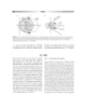
- LEED-Ch-05.qxd 11/27/05 2:21 Page 224 224 Chapter 5 Constructive plate boundary at midocean ridge Eurasia Conservative plate boundary at oceanic North transform fault or continental strike-slip America fault JF Sense of plate motion across ridge (usually, but not always orthogonal to Ph Ca ridge axis) Pacific Co Destructive plate boundary at trench, Africa South filled barbs on side of overriding plate Indian America Nazca Zone or suture of continent-to-continent collision, unfilled barbs on overthrust terrain Antarctic Fig. 5.35 Outline of major plates. Ca: Caribbean plate; Co: Cocos plate; Ph: Philippine plate; JF: Juan de Fuca plate. assembled much fossil and geological evidence to support approaching the partial melt curve for mantle rock (Section the theory of Pangea and its breakup, including the long- 5.1) that allows the whole process of plate tectonics to known jigsaw-fit of the Atlantic coastlines. Subsequently in operate. The asthenosphere behaves as a high-viscosity (c.4 1019 Pa s) fluid in this scheme of things. Plate thick- the 1920s Holmes postulated a thermal mechanism for continental drift that involved the continents moving ness varies according to whether continental or oceanic above convection currents in the mantle. Powerful opposi- crust is involved in the upper layers; oceanic plate thickens tion to this notion came from the geophysicist Jeffreys and laterally from zero at the ocean ridge to a maximum of others, who could not accept that the mantle could con- 80 km, while the thickest continental lithosphere may be vect. This gave many skeptical and conservative geologists greater than 200 km. It is a key fact that, unlike the isosta- the excuse to ignore the theory. Major breakthroughs tic equilibrium of crust and mantle (Section 3.6), oceanic came with the development of paleomagnetism (study of lithospheric is denser than the underlying asthenosphere. the ancient magnetic field recorded by magnetic particles This inverted density stratification leads to the production in rock) and seismic exploration of the ocean basins after of negative buoyancy forces, which drive plate destruction World War II. The key developments were: by subduction at the oceanic trenches. 1 A record of diverging magnetic pole positions for different sites over Pangea indicating that continental drift had defi- 5.2.2 A brief historic overview nitely occurred, though many did not believe the new science of paleomagnetism for several years after the mid-1950s. 2 A record of geomagnetic field reversals (magnetic north It is instructive to briefly review the development of plate and south switching for long periods) in continental rocks tectonics because the logic developed to account for vari- dated precisely by radiometric dating. ous key components comes from a range of subject areas: 3 Global mapping of midocean ridges and oceanic trenches. paleontology, paleoclimatology, geology, geophysics, and 4 An oceanic record of normal and reversed fields geochemistry. Alfred Wegener, a meteorologist by train- recorded in linear magnetic anomalies that lie symmetri- ing, developed his theory of continental drift in 1915 cally about the midocean ridges (Fig. 5.36): this led to the starting from the basis that a supercontinent called Pangea Vine–Mathews theory of sea-floor spreading in 1963. (Greek: “all Earth”) progressively broke up over c.250 5 The seismological recognition and significance of the million years (My) into today’s separate continental LVZ (Sections 1.5 and 4.17) in defining the mechanical masses. Wegener and later du Toit (Wegener tragically layers of lithosphere and asthenosphere. died during an Arctic meteorological expedition),
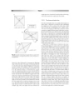
- LEED-Ch-05.qxd 11/27/05 2:21 Page 225 Inner Earth processes and systems 225 (a) PLATE A UA = UB Ridge UA A A A B UB Transform UA UB Ridge A B B Transform UA UB Ridge A A B PLATE B (b) Transform fault with Spreading UA = 0 earthquake ridges UB locii Ocean floor fracture zone with no relative strike slip motion (old transform trace) UB Velocity vectors defining velocity field for B plates A and B. Fig. 5.37 Sketch to illustrate ridge : transform relationships between UB two moving plates. Fig. 5.36 Sea floor spreading is a continuous process; magnetic min- 11 Identification by Forsyth and Uyeda of the “self- erals in the oceanic lithosphere record the orientation of the mag- propelled” theory of plate driving forces, chiefly involving netic field that existed at the time of solidification. Here, the black slab pull. shading depicts periods of normal magnetic polarity and the white shading reversed polarity. (a) Shows the conventional view of sym- metrical spreading about a fixed midocean ridge axis, (b) shows an alternative scenario in which plate A is held fixed and the spreading 5.2.3 Magnitude of plate motion: Rates of sea-floor ridge migrates away from it at half the spreading rate. In both cases, spreading and other statistics a symmetrical pattern of magnetic anomalies results. Sea-floor spreading is the evocative name given by Vine and 6 Recognition of the particular structural features of a Mathews in 1963 to the discovery that midocean ridges type of oceanic strike-slip fault, termed a transform fault were the center of creation of ocean crust. They were able to (Fig. 5.37). say this because accurate shipboard magnetic surveying 7 Identification of Benioff–Wadati zones of deep earth- revealed geomagnetic reversals as symmetrical strips of nor- quakes along tilted interfaces under the oceanic trenches; mal and reversed ocean crust situated either side of the 8 the seismological recognition of plate boundaries along ridges (Fig. 5.36). The accurately dated continental record (1) midocean ridges (extensional first motion earthquake of reversals was already established and it was then possible mechanisms), (2) subduction zones (compressional first to correlate the oceanic record with this and to establish the motion earthquake mechanisms). precise time of creation of known widths of ocean crust, 9 The McKenzie–Parker kinematic theory of “tectonics something eventually traceable over 150 My. The speed of on a sphere” (simply defined in Fig. 5.38) from magnetic present plate motion, mostly derived from this sea-floor anomaly and transform fault data, with the concept of spreading data, varies over about an order of magnitude, from 11 to 86 mm y 1. The speed of motion is related to Euler poles of rotation. 10 The parameterization of a Rayleigh Number (Section the magnitude of the driving forces and resisting forces asso- 4.20) well above critical for the existence of convection in ciated with particular plates. Table 5.1 gives relevant the asthenospheric mantle. statistics for the major plates and some of the minor ones.
- LEED-Ch-05.qxd 11/27/05 2:21 Page 226 226 Chapter 5 (Figs 1.9, 4.109, and 4.142), Dead Sea fault, Jordan (Fig. 4.110), and North Anatolian fault (Fig. 2.16). sform Tran In all the above examples, we discussed the nature of r binary plate boundaries, that is, where two plates meet. However, it is theoretically possible to imagine multiple PLATE B u AB junctions meeting at topological points. In fact, points where three plates meet, termed triple junctions, are the Sp u rea most common. These involve various combinations of AB e on din ridge, trench, and transform boundaries. The interesting nz gr tio idg thing about them is that they may migrate with time. uc e u bd AB Su 5.2.5 Describing the kinematics of plate motion – . plate vectors, Euler poles, and rotations on a sphere Euler rotational pole u =u ω Since we all live on one of the moving plates, any state- AB B A PLATE A ment concerning the directional vectors of the motion we undergo year upon year must be done with care. A vivid Fig. 5.38 Sketch to show Plate B rotating with respect to Plate A. example comes from kinematic representations of the sym- Plate is generated at the spreading ridge and rotates as a solid body metrical pattern of sea-floor magnetic anomalies. about circular arcs. The northern boudary to Plate B is a transform Figure 5.36 shows the usual explanation for this, that of fault, an orthogonal line from which defines a great circle upon which the Euler pole lies. The linear velocity vectors are the velocities symmetrically diverging plates with equal speeds but of Plate B moving with respect to Plate A. The length of the arrows opposite directions, that is, uA uB. In fact, the sym- is proportional to velocity magnitude which varies with the rotational metrical spreading can equally well be achieved by motion radius, r, about the Euler pole shown. A typical angular velocity, , is of plate B, with plate A fixed, as long as the spreading axis about 10 8 radians per year. also migrates in the direction of B at a velocity of 0.5Bu. This kind of relative motion is entirely possible since plates 5.2.4 Plate boundaries, earthquakes, and volcanism are self-driven entities and spreading ridges do not have to overlie upwelling limbs of convection cells fixed in asthenospheric mantle space. Plate boundaries are described as constructive when new We may most generally express plate velocities as relative oceanic plate is being added by upwelling asthenospheric velocities, that is with respect to adjacent plates, which have melt at the midocean ridges. Remember that this melting is boundaries with the plate in question; Fig. 5.38 shows a due to adiabatic upwelling of mantle peridotite (Section 5.1). simple two-plate example where the velocity of plate A with The volcanism is accompanied by voluminous outpourings respect to plate B is minus the velocity of plate B with of hot fluids along hydrothermal vents (Section 1.1.3). respect to plate A, that is, BuA AuB. To do more com- Shallow and relatively minor normal faulting (extensional) plicated three-plate problems, we can use the techniques of earthquakes accompany this plate creation along the ridge vector addition and subtraction (Fig. 5.39). Sometimes a axis. Destructive boundaries occur at the ocean trenches fixed internal or external reference point is used to express where plate is lost to the deep mantle by subduction. the plate velocity vector. It is generally held that certain The process is manifest by arrays of deep earthquakes “hot-spots,” the surface expressions of rising mantle (Section 4.17) along Benioff–Wadati zones and below plumes (the Hawaiian islands are the best known example) island arcs. These latter form as water from the descending may approximate to such stationary points. Another trick slabs dehydrate the water fluxing mantle of the overriding relevant to some geographical situations is to fix one plate plate so that the mantle geotherrn intersects the peridotite and relate other plate velocities with respect to that. solidus (Section 5.1). Conservative boundaries are those The linear speed, u, of any rotating plate on the spherical where no net flux of mass occurs across them, the plates surface of the Earth is a function of both angular speed of simply slide past each other. In the oceans this occurs the motion and the radius of the motion, r, from its rota- along the active parts of oceanic fracture zones, called tional pole, the linear speed increasing as the length of the transform faults (Fig. 5.37). Strike-skip faults in continen- arc increases (Fig. 5.38). Linear speed is thus given simply tal lithosphere may also mark conservative plate bound- by u r . The rotational pole is commonly termed the aries; examples are the San Andreas Fault, California
- LEED-Ch-05.qxd 11/27/05 2:22 Page 227 Inner Earth processes and systems 227 Table 5.1 Plate statistics, see Fig. 5.35 for map. Asterisked plates have long trench boundaries and are fastest due to the importance of slab pull forces in generating steady plate motion (see Section 5.2.7). Plate Total area Land area Speed Periphery Ridge Trench 106 km2 106 km2 1 102 km mm year length length 102 km 102 km NA 60 36 11 388 146 12 SA 41 20 13 305 87 5 PAC* 108 0 80 499 152 124 ANT 59 15 17 356 208 0 IND * 60 15 61 420 124 91 AF 79 31 6 418 230 10 EUR 69 51 7 421 90 0 NAZ* 15 0 76 187 76 53 COC* 3 0 86 88 40 25 CAR 4 0 24 88 0 0 PHIL* 5 0 64 103 0 41 ARAB 5 4 42 98 30 0 ANATOL 1 0.6 25 28 0 8 Plates: NA – North America, SA – South America, PAC – Pacific, ANT – Antarctica, IND – India, AF – Africa, EUR – Eurasia, NAZ – Nazca, COC – Cocos, CAR – Caribbean, PHIL – Phillipine, ARAB – Arabian, ANATOL – Anatolian. –40 V BA Plate A Plate A V AB +40 +40 V Plate C AB V C A +30 Plate C V = +50 CB V V –30 +30 CA AC Plate B Plate B Fig. 5.39 There are three plates and alleline. The velocities of A and B and A and C with respect to each other (in millimeter year 1) are known. We want to know the velocity of B with respect to C. This is given by vectorial addition, as shown on the right. Velocity vector codes like BVA read “the velocity of A with respect to B.” Euler pole and is most easily found by drawing orthogonal advecting mantle generates heat at the ridge due to adia- lines from transform faults (see below), the latter being arcs batic decompression. The associated melting produces of small circles on the global sphere. The Euler pole is on a new oceanic crust at the ridge axis and defines a thermal great circle perpendicular to the trend of the transform fault. boundary layer in the form of cooling plate mantle that thick- ens away from the point of upwelling. It is thus axiomatic that lithospheric mantle above the top-asthenospheric 5.2.6 Thermal aspects of plates and slabs 1,000 C isotherm must gradually thicken laterally due to conduction of the adiabatic heat released out through the upper surface of the new ocean crust into the ocean Consider first of all the likely temperature distribution in (Fig. 5.40). We ignore here the undoubted highly efficient the upper 1 km of the lithosphere in a lateral transect from convection witnessed at the ridge axis by hydrothermal the mid-Atlantic ridge in Iceland to New York. At the systems responsible for “black smokers” (Fig. 3.6). In ridge there is abundant evidence in the form of submarine physical terms, our example means that temperature is volcanic activity and from heat flow measurements that changing with time and distance from the ridge temperatures in the upper crust are high and that overall (Fig. 5.40). However, our most complicated heat conduc- heat flow is high (Fig. 5.40). In the case of offshore New tion scenarios to date (Section 4.18; Cookie 20) say that York the opposite is true. Divergent plate boundaries, like T only changes with distance! Advanced sums (hinted at in this North Atlantic example, obey the simple rule that an
- LEED-Ch-05.qxd 11/27/05 2:22 Page 228 228 Chapter 5 x=0 x t= (a) 250 (c) T = T0 ridge u q q q 200 T = T1 u u u 150 q0, (mW m–2) t = t0 t = t1 t = t2 t (Myr) 100 (d) 0 50 100 150 0 200 400 50 50 600 z (km) 800 100 1000 0 0 50 100 150 200 t (Myr) 150 u (b) Ridge x = 0 T = T0 Surface Lithosphere rm e Isoth T1 Asthenosphere z x Fig. 5.40 Thermal matters for oceanic plate (a) Heat flow oceanwards from a midocean ridge, with distance expressed as plate age (derived from ocean magnetic anomalies). Dots are measurements, curves are various theoretical estimates based on the erfc argument. (b) The mechanical situation, with hot upwelling asthenosphere cooling laterally to define the plate thermal boundary layer above the isotherm at c.1,000 C. (c) The physical situation, with heat flow, q, conducting vertically through the ocean floor from the thickening plate above the c.1,000 C isotherm. q decrease with time and the plate thickens with time according to the erfc argument (see text). (d) The proof of the pudding: data on plate thickness (dots) from seismic surveys versus estimates of plate thickness to the 1,000 C isotherm from heat conduction theory. Cookie 20) tell us that the thickness, zt, of this thermal envisaged is buoyantly unstable is also axiomatic. Also, global boundary layer changes in proportion to the square root continuity tells us that creation of oceanic lithosphere in one of time, t, as the simple expression 2.32 t , where is place must be accompanied by destruction elsewhere if the the thermal diffusivity (Section 4.18.3). The square root Earth is to maintain constant volume. The fate of oceanic term is a characteristic thermal diffusion distance and zt plate is therefore determined; it has to be destroyed. Pushing refers to the thermal boundary layer thickness defined as cold slab into the hot mantle (Fig. 5.41) creates a thermal the thickness appropriate to a base lithosphere tempera- anomaly, that is, the lithosphere is cooler than it should be ture of 90 percent of steady state value c.1,000 C. for the depth it has reached. This has the effect of raising the So, ignoring all the geological differences, we know olivine : spinel transition (Section 4.17.4) by several tens of that the lithosphere can be regarded simply as a cold, dense kilometers in the slab (Fig. 5.41) and creating additional layer lying above warmer asthenosphere. That the situation negative buoyancy that adds to the slab pull force (explained
- LEED-Ch-05.qxd 11/28/05 10:56 Page 229 Inner Earth processes and systems 229 Anomalous mantle Trench (High heat flux) Depth (km) 400ºC 800ºC slab continental lithosphere oceanic 100 dewatering 1,200ºC 1000ºC lith. here Spinel 200 300 P Olivine 1,600ºC 400 Spinel 500 Olivine 600 Spinel T 1,700ºC Perovskite and Magnesiowüstite 700 800 900 Fig. 5.41 A computed estimate of subsurface temperatures achieved as a subducting slab passes down into the lower mantle. The cold slab is denser than the ambient mantle and, despite the production of heat due to shearing along its upper interface, retains its identity to very great depths before it merges thermally with the lower mantle. Note that the olivine to spinel phase change is elevated in the descending slab and the dense spinel phase occurs at shallower depths here. The combination of cool, dense slab and elevated spinel transformation supplies the negative buoyancy necessary to drive the steady slab descent as a “slab-pull” force. in Section 5.2.7). Also, as we have previously discussed The topography has a thermal origin since it is due to the (Section 5.1.4), volcanoes occur in volcanic arcs, not because buoyancy of upwelling hot asthenosphere (including some of frictional melting, but because massive loss of water from partial melt), which underlies it (the Pratt-type isostatic dehydrating slab mantle serpentinite at c.150 km depth. compensation discussed in Section 3.6). Top forces are also possessed by the continental lithosphere, for the high- est mountains lie up to 9 km above sea level. Potential 5.2.7 Why do plates move? The forces involved energy possessed by such elevated terrain may be liberated as kinetic energy if the terrain in question can be decou- Individual plates appear to be in steady, though not neces- pled from its rigid surroundings, that is, by basal sliding sarily uniform, motion. The steadiness means that acceler- and along peripheral strike-slip faults. The Tibetan plateau ations causing inertial effects are absent and therefore by is a case in point. Here the plateau, average elevation 5 km, Newton’s Second Law all relevant forces must be in bal- lies above a very weak lower crust (probably due to a small ance. The occurrence of nonuniform motion is evidenced degree of partial melting) and the whole area is collapsing by results from satellite GPS surveys of the continental outward, by basal sliding rather like a crustal glacier. At the lithosphere (see Fig. 2.16). It means that, although rigid, same time it is extending by normal faulting at the surface. plates can strain internally by elastic deformation as part of Another example is the Anatolian–Aegean plate the cycle of stress buildup and release associated with (Fig. 2.16), which is being shoved outward due to the earthquake generation. The forces in equilibrium that energetic impact of the Arabian plate into the Iraq/Iran drive plate motion (Fig. 5.42) may be divided into top part of the Asian plate along the great Zagros thrust fault. forces that act because of differential topography, Anatolia–Aegea is decoupling (“unzipping”) along the edge forces that act on peripheral plate boundaries, and North Anatolian strike-slip fault, allowing the stored basal forces that act on the bases of plates. potential energy of the Anatolian Plateau, some 5 km Top forces arise from the potential energy available to above the deep Hellenic trench, to be released. topography. For example, the midocean ridges lie several Edge forces result from a number of mechanisms. The kilometers above the abyssal plains. A force, termed ridge- chief one that seems to provide the major driver for plate push, is thus pushing the plate outward from the ridge. motions is that of slab-pull. This arises as a negative buoyancy
- LEED-Ch-05.qxd 11/27/05 2:22 Page 230 230 Chapter 5 Ridge Continent Fts Trench Frp Plate Fcd b Sla wedge Fadf For steady plate motion Asthenosphere driving forces = resisting forces Fsd Fsp Fsp + Frp = Fsd + Fcd + Fadf Fsd Fig. 5.42 The major forces involved in determining steady plate motion. Fsp – slab pull force; Frp – ridge push force; Fsd – slab drage force; Fcd – collision drag force; Fadf – asthenospheric drag force. Fts is the trench suction force, which acts to cause oceanward movement of the overriding plate if the slab should retreat oceanwards. a large-scale underlying circulation of the asthenosphere; a force because, as we mentioned before, a subducting slab form of forced convection or advection (Section 4.20). of oceanic lithosphere is cooler and denser than the Overall, calculation of the various torques acting upon asthenosphere in which it finds itself. It thus sinks at a the major plates shows that the slab pull force, balanced by steady rate (remember Stoke’s law, Sections 3.6 and 4.7) the basal slab resistance force, is the major control upon until it reaches some resisting layer within the earth or it steady plate velocity and the slab resistance force is greater heats up, melts, or otherwise transforms so that the buoy- under continental plate areas than oceanic areas. This cor- ancy is eventually lost. Another edge force arises when a relates with the known speeds of plates, those oceanic plates subducting plate moves oceanwards by slab collapse under attached to subducting slabs being faster (Table 5.1). an overriding plate. A suction force drives the overriding plate oceanwards, causing strain, stretching, and the for- mation of back-arc basins like the Japan Sea. Resisting edge 5.2.8 Deformation of the continents forces are the frictional resisting forces that exist along plate peripheries, including transform fault friction, strike-slip Although the oceanic and continental lithosphere are both fault friction, slab drag resistance, and for some deeply rigid, the latter is not particularly strong; many areas are penetrating slabs, slab end resistance. being strained due to the effects of adjacent or far-field Basal forces have historically been the most controversial forces. of driving mechanisms for it was the role of thermal convec- First, we consider extensional deformation. We turn tion (Section 4.20) in basal traction that was the first again to the eastern Mediterranean (Fig. 5.43) to illustrate proposed mechanism to drive continental drift by Holmes this since it contains the best known and fastest extending and others. While there is little doubt that asthenospheric area of continental lithosphere in the world, Anatolia– convection occurs, there seems little likelihood that basal Aegea. At the leading edge of this plate we saw earlier traction along a convecting boundary actually drives the (Fig. 2.16) that a spatial acceleration can be picked up in plate motion. This is because the almost 1 : 1 aspect ratio of the Aegean region, with the largest rate across the Gulf of Rayleigh–Benard convection cells (Section 4.20) is com- Corinth. You can see this in Fig. 2.16 by closely compar- pletely unsuitable to provide plate-wide forces of sufficient ing the vectorial velocity field arrows to the south and net vector: many such cells must underlie larger plates like north-east of the gulf, the velocity increases by more than the Pacific and their applied basal forces would largely cancel 30 percent, about 10–15 mm yr 1. Now although the when integrated over the whole lower plate surface. Basal whole region contains a great number of normal faults and resisting forces due to asthenospheric drag are much more it is evident that local strains of smaller magnitude may certain, for the motion of a plate must meet with viscous cause earthquakes and fault motion, the great majority of resistance over the whole lower plate surface. In this scheme, strain energy is being released along the particular array of the asthenosphere passively resists motion; continuity simply normal faults that define the southern margin to the Gulf requires the mass of the moving plate to be compensated by
- LEED-Ch-05.qxd 11/27/05 2:22 Page 231 Inner Earth processes and systems 231 (b) 38º 12' x ALKYONIDES GULF 38º 08' 5.0 km --- - +++ - x´ ++ -- + - - - -Skinos - - - Abandoned, 38º 04' -- - uplifting and incising rift basin 38º00’ Loutraki N (a) Corinth 37º 56’ 40º NAF E. Mediterranean ANATOLIAN SARONIC GULF PLATE 23º 05' 22º 50' 23º 10' 22º 55' 23º00’ 23º 20' 38º B. Major active offshore and onshore faults + Uplifting late-Quat.-Holocene coastline - Subsiding late-Quat.-Holocene coastline He l le ni (c) 36º c 33 mm/yr x´ x ub s du Mean sea level 0.04 ms TWT 6 mm/yr ctio n Last (70–12 ky BP) Major zo lowstand shoreface n 34º AFRICAN PLATE e Minor active deposits fault fault Holocene 20ºE 23ºE 26ºE Debris lobe Submarine Volcanic centres of Aegean volcanic arc fan Progressive onlap of hangingwall dipslope Basin-fill sediments Pre–rift basement Prominent reflectors corresponding to sedimentation during highstands of sealevel Fig. 5.43 Deformation of the continental lithosphere: Extension across the Gulf of Corinth rift, SW Anatolian–Aegea plate. (a) Context of plate, with active plate boundaries along the North Anatolian strike-slip fault (NAF) and the Hellenic subduction zone. (b) Detailed DEM to show relief and faulting associated with the active coastal fault system in the eastern rift. In this area the fault footwalls are uplifting and the hangingwalls subsiding. The dashed line x–x is the line of section of C. (c) An interpreted seismic reflection survey line, x–x , showing the tilted, half-graben form of the Alkyonides gulf. The Two Way Time (TWT) scale in milliseconds indicates time taken for seismic energy to pass from sea surface source to depth and back again to a receiver. Maximum water depth here is about 300 m.
- LEED-Ch-05.qxd 11/27/05 2:22 Page 232 232 Chapter 5 of Corinth (Fig. 5.43b). The huge strains accompanying G crustal thickening and buoyancy enhancement of the this differential motion are released periodically along crust by the wholesale intrusion of lower density calc-alkaline powerful earthquakes on these faults (the seismogenic magmas as plutonic substrates to volcanic arcs; layer here ranges from 10 to 15 km thick). The Corinth G whole-lithosphere thickening into a lithospheric mantle gulf is termed a rift or graben. In the east, a half-graben for “root” by pure strain, manifest at crustal levels by shear the normal faults that define it are only on one side, strain along major thrusts; causing the prerifting crust to tilt southwards into the G buoyant up thrust of crustal mass in thickened faults (Fig. 5.43c). Detailed GPS surveys also reveal that lithosphere resulting from the wholesale detachment of the southwest Greece is rotating anticlockwise with respect lithospheric mantle root; to the motion of the northern area. This illustrates that G gravitational collapse of the elevated plateau with release plates have vorticity, that is, they can spin as solid bodies of gravitational potential energy along active normal faults. about vertical axes. The continental lithosphere may also deform under 5.2.9 The fate of plates: Cybertectonic recycling extension over vast areas, exemplified by the high (greater and the “Big Picture” than 2 km) plateau of the western United States and adja- cent areas of Mexico. The plateau is known as the Basin and Range on account of the myriad of individual normal Three possible scenarios concerning the large-scale recy- fault-bounded graben and half-graben that make it up cling of plates have been envisaged at different times since (Fig. 5.44). The individual ranges are the uplifted footwall the plate tectonic “revolution” in the late 1960s; they are blocks to the normal faults (Section 4.15) while the basins sketched in Fig. 5.46. are the sediment-filled depressions, subsiding hangingwall 1 A system of whole-mantle convection in which plates are car- ramps between the ranges. Range wavelengths are typically ried about by applied shear stress exerted at their bases by the 5–15 km with lengths up to several times this. Today the convecting mantle. The plates are thus part of a whole-mantle GPS-determined velocity field in areas like Nevada is east plate recycling system. The irregularity of plate areas and vol- to west at about 20 mm year 1 with respect to fixed east- umes compared to the regular system of convecting cells in ern North America. The active normal faulting is located Rayleigh–Benard convection (Section 4.20) is a problem with in distinct belts of high strain at either side of the province, this idea. Also, the scheme requires rather wholesale mixing of chiefly associated with the Central Nevada Seismic Belt in slabs into the ambient mantle to prevent any lithospheric the transition to the more rapidly northwest-moving chemical signature contaminating the very uniform melt com- California terrain, and to a lesser extent along the western positions represented by midocean ridge basalts (MORB). margin to the Wasatch front in Utah. Although historic 2 This recognizes a fundamental physical discontinuity in earthquakes have nucleated along steeply dipping normal the mantle at a depth of about 660 km due to the phase faults (Fig. 5.44b) bounding individual range fronts, there change of the mantle mineral spinel to a denser perovskite is a record in the tectonic landscape of a previous phase of structure. A two-tier convection/advection system is envis- low-angle normal faulting (Fig. 5.44c,d). The kinematics aged, involving largely isolated lower mantle convection of this kind of extension has given rise to areas of core- cells below the 660 km discontinuity. The upper mantle complexes, mid- to lower crustal rocks exposed in the tier comprises a separate advecting system with plates footwalls to the low-angle faults. It is thought by some driven by the edge- and top-forces discussed previously and that this phase of low-angle faulting was related to a very with no slab penetration into the lower mantle. Separation rapid gravitational “collapse” of the over thickened Rocky of the lower and upper mantle in this way, with plate recy- Mountain crust some 20–30 Ma, with associated high- cling restricted to the upper mantle, might be expected to heat flow and volcano-plutonic activity. gradually change the composition of the MORB through Shortening deformation of the continents under time. The scheme does not allow for the buoyant penetra- compression occurs at plate destructive and continent– tion of lower mantle plumes into the upper mantle and continent collision boundaries where five physical processes crust. The scheme was originally supported by the lack of occur, often combined or “in-series,” that cause the forma- slab-related earthquake hypocenters below 660 km. tion of linear mountain chains like the Pacific arcs, the 3 This is really a hybrid scheme that has received a degree Andes, and the Alpine-Himalaya (Fig. 5.45) system: of acceptance in recent years. It involves both ongoing G crustal accretion by thrust faulting (see discussion of thrust lower mantle convection, upper mantle advection with duplexes in Section 4.15) of trench sediments “bulldozer-style” plates driven by edge- and top-forces and periodic slab against the overriding plate – this results in the formation and penetration below the 660 km discontinuity. The model rapid uplift of an accretionary prism; arose in the 1990s as advances in seismic tomographic
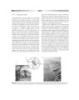
- LEED-Ch-05.qxd 11/27/05 2:22 Page 233 Inner Earth processes and systems 233 (b) (a) 50º 40º San Andreas fault USA 30º (c) Legend Normal faults Strike-slip fault Core complexes Mx 20º Motion direction 500 km during extension 120º 110º 100º (d) Fig. 5.44 Extensional tectonics of the western United States. (a) Map shows huge extent of the Basin and Range province with its arrays of normal faults and the location of the chief core complexes. Star indicates the site of the 1985 Borah Peak normal faulting earthquake. Large shaded arrows indicate the direction of extention revealed by the normal faults bounding the core complexes. (b) Field photo of part of the impressive surface fault break of the Borah Peak earthquake. Mike is standing on the uplifted footwall block, facing the subsided hangingwall block; total displacement is some 3.0 m. (c) and (d) show sequential development of a core complex due to a period of rapid, high exten- sional strain causing unroofing and uplift of mid-lower crust along a major low-angle crustal detachment normal fault system (to right of pointer).
- LEED-Ch-05.qxd 11/27/05 2:22 Page 234 234 Chapter 5 33 km thick crust Gangdese (a) Late Cretaceous (70 Ma). Indian oceanic plate subducting under the Asian continent, scraping off Xigatse oceanic sediments and creating the Gangdese magmatic arc to the north Tsangpo suture (b) Middle Oligocene (36 Ma). 65 km Indian continental lithosphere collides with Asia to create Tsangpo suture; lithospheric thickening propagates north; sediment provided by denudation of the nascent Himalaya is deposited in the thrust-fault bounded sedimentary basins to the north and south Main Boundary (c) Middle Miocene (11 Ma). Tibetan Thrust fault Plateau at c.3 km elevation above thickened lithosphere; active shortening results in widespread 33 km thrust faulting across Plateau with strike-slip faulting at northern margin km 65 (d) Pleistocene (1 Ma). The thick 2 km lithospheric “root” under the Tibetan Plateau sinks into the asthenosphere causing rapid and regional uplift to c.5 km mean elevation. Whole Plateau begins to extrude laterally, releasing gravitational potential energy by widespread normal faulting Fig. 5.45 Continental shortening deformation on a grand scale: development of the collision of the Indian and Asian plates along the Himalayan mountain belt and the uplift and sideways collapse of the high Tibetan Plateau.
- LEED-Ch-05.qxd 11/27/05 2:22 Page 235 Inner Earth processes and systems 235 processing enabled geophysicists to track the fate of gested that mantle plumes and therefore large-scale out- descending cool slab down to and often through the once bursts of intraplate continental magmatism might arise inviolate 660 km discontinuity. This was linked to the abil- from periodic “eruption” of molten slab at this boundary, ity of seismologists also at this time to distinguish what was though there seems little evidence that core material itself interpreted as slab material at or about the core-mantle is involved in this process. It seems that Cybertectonica acts boundary, a zone termed “D”. These developments sug- from surface to core/mantle boundary. (b) (a) core core (c) Hawaii Pacific Rise le t an rM pe Up core Africa Fig. 5.46 Models for plates, plumes, and mantle convection. (a) Whole mantle convection drives and recycles plates. (b) Two-tier system with plate advection and lower mantle convection separate. (c) Upper level advection with deep slap penetration, periodic plume upwelling and lower mantle convection.
- LEED-Ch-05.qxd 11/27/05 2:22 Page 236 236 Chapter 5 Further reading and in E.M. Moores and R.J. Twiss’s Tectonics (Freeman & P. Francis and C. Oppenheimer’s Volcanoes (Oxford, 2004) is Company, 1995). The bible for advanced solid Earth studies the most accessible account of volcanoes. For a comprehen- of melting, stress, strain, and general dynamics from the point sive and practically orientated overview of plate tectonics of view of mathematical physics is the unrivalled Geodynamics from the very basics, nothing can beat A. Cox and by D.L. Turcotte and G. Schubert (Cambridge, 2002). R.B. Hart’s Plate Tectonics; How it Works (Blackwell, 1986). Probably the best intermediate level text is C.M.R Fowler’s Comprehensive, stimulating, and accessible accounts are The Solid Earth (Cambridge, 2005). P. Kearey and F. Vine’s Global Tectonics (Blackwell, 1996)
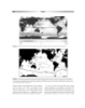
- LEED-Ch-06.qxd 11/27/05 2:30 Page 237 6 Outer Earth processes and systems 6.1 Atmosphere 6.1.1 Radiation balance and heat transfer formation of clouds and the precipitation/evaporation of surface waters (latent heat transfer). Thus although the troposphere away from the tropics is in radiation deficit It is important initially to consider the net balance of (Fig. 6.2), the overall positive net radiation from the incoming solar radiation energy and outgoing reradiated Earth’s surface due to the greenhouse effect (Section 4.19) energy from Earth over a long time period. We need to means that the planet is in balance due to this transfer of consider energy transformations also, like those between heat from low to high latitudes by oceanographic and tro- conductive and convective heat energy, potential and pospheric circulation. To illustrate this, imagine that kinetic energy. In Fig. 6.1, 100 units of energy represent Earth, like its Moon, has no atmosphere. Then at any one the magnitude of the incoming shortwave solar radiation time there would be a perfect energy balance between flux (sometimes termed insolation) at the outer atmos- incoming shortwave insolation to the side of Earth facing phere; because of the Earth’s planetary albedo, approxi- the Sun and outgoing longwave reradiation from the mately 32 percent of this is reflected back into space. Of whole Earth. The mean surface temperature would then this total reflection, about 23 percent is from clouds behav- be about 254 K, or 19 C. This compares to the actual ing as perfect blackbodies and about 9 percent is directly mean surface temperature of around 14 C. The surplus from Earth’s surface. This reflected radiation plays no part temperature of 31 C is due to the greenhouse effect, in the climate system. The remaining incoming radiation is whereby Earth’s atmospheric gases absorb, reradiate, either absorbed by the Earth’s surface as direct and diffuse and reabsorb significant portions of the outgoing infrared radiation (~49%) or absorbed by the atmosphere and radiation from the surface and make this energy available clouds (~20%). Note the smaller atmospheric absorption for the lateral and vertical transport of heat energy by the compared with the large surface absorption. As seen previ- troposphere. It is only in dry desert areas that the Earth’s ously (Section 4.19), the latter is converted into heat climate is dominated by radiative exchanges alone, with energy and, by Wein’s law, is reradiated into the atmos- high daily and low nightly temperatures. phere as longwave radiation, where most of it is absorbed The result of tropospheric heat transfer processes is a and then reemitted (at the same wavelengths). More long- mean thermal structure shown in Fig. 6.3. The warmest wave radiation in net terms is lost to space in this process temperatures, about 27 C, are at lowest latitudes, from the troposphere (~60%), chiefly from cool cloud tops, decreasing toward the poles and vertically up to the top of than is absorbed (~17%). Together with the 19 percent of the tropopause at between 10 and 15 km elevation. The shortwave radiation absorbed, this means that there is a troposphere is thickest at low latitudes, thinning toward total absorption deficit of more than 35 percent. the poles. The greatest vertical and lateral gradients of T Should the matter rest there, the Earth’s troposphere occur toward the top of the troposphere, a prominent and surface would cool drastically, to below 0 C. So, boundary within the overall temperature structure of the where does the “extra” energy come from? The deficit is whole atmosphere. Note that in general, particularly away provided by the transfer of heat energy from the Earth’s from the tropics, the isotherms controlling air density surface by conduction and convective turbulent exchange diverge from the major latitudinally (zonally) averaged, (called sensible heat transfer) and as a by-product of the
- LEED-Ch-06.qxd 11/27/05 2:31 Page 238 238 Chapter 6 Incoming Outgoing radiation radiation 100 units OUT 100 units IN short short wavelength Long wavelength Space wavelength 68 32 Absorption Stratosphere by 03 Backscatter 23 by 9 Absorption Emission by H2O, clouds by atmosphere CO2 , and clouds Backscatter and clouds 19 Absorption Heat transport by Troposphere atmospheric mixing back Dust, aerosols Latent Sensible reflection heat heat in thermals 49 Hydrosphere Net longwave Absorption of Absorption of Lithosphere reradiation Heat transport by direct solar + diffuse sky and ocean currents radiation cloud radiation Fig. 6.1 Energy transport in and out of the atmosphere. +80 ause op Trop 190 210 +40 Net radiative flux (W m–2 ) 210 200 230 Surplus 240 0 250 Pressure (mbar) 400 Deficit 260 –40 270 600 –80 280 800 –120 290 90N 60 30 0 30 60 90S 1000 Latitude (degrees) 90N 60 30 0 30 60 90S Fig. 6.2 Net annual zonally averaged radiative flux (shortwave Latitude (degrees) absorbed flux minus outgoing longwave flux) from the top of the Fig. 6.3 Zonally averaged atmosphere temperature ( K) from equa- atmosphere. tor to pole according to a global climate model based on sea-surface temperatures over a 10-year period. Note the vertically persistent equator-to-pole temperature gradient, its decrease with altitude, and equal-pressure surfaces (isobaric surfaces): in other words, the poleward thinning of troposphere. Also note strong baroclinicity the baroclinic condition (Section 3.5) dominates. away from equator (see discussion of “thermal wind”). 6.1.2 Thermal wind, pressure gradients, and origin of large-scale global circulation gradients from equator to pole and (ii) strong vertical density gradients set up by differential thermal heating and The most fundamental features governing global atmos- cooling of land and sea in equatorial latitudes. We consider pheric circulation (GAC) are: (i) strong negative thermal feature (i) here and (ii) in a later section.
- LEED-Ch-06.qxd 11/27/05 2:31 Page 239 Outer Earth processes and systems 239 Geopotential heights y1 z1 > y2 z1 y1, z3 z y1 z2 > y2 z2 y1 z3 > y2 z3 p3 y2 , z3 Geostrophic winds Ug3 Ug1 < Ug2 < Ug3 p2 x y1 Ug2 p1 y2 r ato Equ Warm Ug1 air column Cold air column North Pole y Fig. 6.4 Definition diagram to aid explanation of the thermal wind concept. p1 are pressure surfaces and their geopotential heights at 3 positions y1 and y2 are y1z1 3 and y2z1 3 respectively. With reference to definition diagram Fig. 6.4, the (a) 1020 Pressure hPa height of a particular pressure surface above sea level is mpsl 1010 termed the geopotential height. Differences in vertical sep- 1000 aration (thickness) between given isobaric surfaces are due to temperature for any given pressure drop. This comes 990 out of the hypsometric equation for layer thickness, z 80S 60 40 20 0 20 40 60 80N (Cookie 7). In warm air columns the layers thus have Latitude greater thickness than those in cold ones, the cumulative Wind speed m s–1 (b) effect of layer-upon-layer of thickening leading to an 6 Westerlies increasing slope of the isobars with height. For the case of 4 2 a negative poleward thermal gradient, we take as reference 0 2 the latitudinally averaged pressure surface low in the tro- Easterlies 4 posphere, say at 1000 mbar, more-or-less at sea level. 60S 40 20 0 20 40 60N Measurements here (Fig. 6.5a,b) show little overall hori- zontal meridional pressure gradient, that is, the average Fig. 6.5 (a) Global meridional transect of mean annual zonal poleward pressure has no large systematic changes other pressures at sea level. Note influence of Antarctica and the southern Ocean. (b) Corresponding mean air speeds. Note the inverse than those across the southern ocean and between the relation to pressure gradient in Figure 6.4. Azores High and Iceland Low (see weather chart of Fig. 3.21). This means that the whole mass of tropospheric both summer and winter, the gradient with height air that exerts the near-sea-level pressure field is distributed decreasing further poleward in both seasons and equator- about uniformly. Now take another pressure surface at ward from about 30 N in summer. Generally the air below 500 mbar in the middle of the troposphere where the air a certain average isobar at the equator is warmer than above is much less dense (Fig. 6.4). The pressure surface the corresponding high-latitude air below the same isobar. falls appreciably (of the order of 10–15%) due to the pole- The differential vertical expansion due to this means that the ward temperature gradient through 40–60 N latitude in poleward thermal gradient is accompanied by a horizontal
- LEED-Ch-06.qxd 11/27/05 2:31 Page 240 240 Chapter 6 hydrostatic pressure gradient (Section 3.5.3) that increases roughness, the flow approximating to that of the vertically from virtually zero close to sea level to a maxi- geostrophic wind set up due to synoptic pressure or tem- mum toward the top of the troposphere at latitudes perature gradients. Such a wind drives flow in the atmos- 50–60 N. The overall concept of this thermal–wind rela- pheric boundary layer (ABL), but because of the effects of tionship is illustrated by comparing the slopes of average surface friction the effectiveness of the Coriolis force in isobars low down and high up in the troposphere. The turning the geostrophic wind markedly decreases; for a increasing slope of the equal pressure surfaces and there- northern hemisphere wind the direction of the frictional fore the increasing strength of the resulting geostrophic wind backs anticlockwise toward the surface, while in the wind (Fig. 6.6) is evident. The thermal–wind relationship southern hemisphere the frictional wind veers clockwise. In thus refers to a rate of change of wind velocity with height; both cases the winds tend to progressively diverge from that is, it is a measure of geostrophic wind shear. The mag- their geostrophic course parallel to isobars through the nitude of the vertical wind shear is directly proportional to ABL. This is known as the Ekman spiral effect (see discus- the horizontal temperature gradient. The high-level wind sion in Section 6.4). The effect of the frictional wind on a strength and its gradient can be mapped as a velocity field low-pressure system is to cause inward spiralling of wind from pressure layer height contour maps. As a geostrophic into the center; this convergence causes compensatory cen- phenomenon (Fig. 6.6) the wind travels parallel to the tral upwelling of air and may cause cloudy conditions as contours of geopotential height (Fig. 6.4) and is faster moist air is cooled and is vice versa for high-pressure systems when contours are closer and vice versa. The maximum when divergence causes central downwelling and clear skies. magnitude of wind shear defines the fast cores of the polar front jet streams that dominate the west-to-east zonal cir- 6.1.4 Energy transformation and the global culation of the planetary wind regime. The jets are atmospheric circulation (GAC) strongest in the winter when temperature contrasts between equator and pole are greatest (Fig. 6.7). In order to understand the principles of the wider GAC, it is now necessary to consider the role of thermal energy 6.1.3 Frictional wind transfer: how energy is transported by a unit mass of moist air. In order to maintain constant total energy, E, in the That part of the wind blowing well above the land or sea face of continuous loss of longwave radiation to space (the may be considered to flow independently of any surface atmospheric radiation deficit earlier discussed), it is neces- sary to add sensible heat from surface land and ocean and from the release of latent heat during rainfall. The general circulations of the atmosphere thus involve a poleward Low transport of heat energy to maintain the observed long- term temperature distributions, which are approximately constant. The simplest such arrangement possible would Geostrophic wind be a general convective upwelling of warm moist air from High the equatorial regions and its transfer toward the poles, Geostrophic wind cooling by radiative heat loss as it does so, where it even- tually sinks, liberating rain, snow, and latent heat. Such a LOW simple cellular circulation, termed Hadley circulation, has the right principles (Fig. 6.8) but inevitably the Earth’s atmosphere is more complicated, chiefly because of the Constant pressure effects of the Earth’s rotation, and also because of pressure gradient force, dp/ds effects due to latitudinal variation in thickness of the tro- posphere. Atmospheric air masses continuously move Coriolis acceleration around and at the same time energy is continuously being Resultant wind transformed from one form to another. Neglecting the very small kinetic energy of air masses, the following forms Fig. 6.6 A starting geostrophic wind begins to flow from high to of energy are involved (Fig. 6.9): low pressure along the constant pressure gradient, dp/ds, but it is 1 Latent heat energy, EL, arises in moist air from reversible progressively and increasingly turned due to the Coriolis accelera- phase changes of state between liquid, water, and gaseous tion (shown here for the southern hemisphere).
- LEED-Ch-06.qxd 11/27/05 2:32 Page 241 Outer Earth processes and systems 241 25 10 0 Tropopause 10 10 -60 Isovels m s–1 20 20 20 10 -60 Isothermals oC -40 -40 30 Height, km -80 15 20 jet stream The zonal winds are the -60 core strongest component of the jet stream global circulation: you -40 10 core should imagine the winds flowing normal to and out of the plane of section represented by the page 5 0 0 0 westerlies westerlies trades trades 90oS 60oS 30oS 0o 30oN 60oN 90oN Easterlies Easterlies Zonal here refers to wind flow normal to a circumferential section from North pole to South pole, showing the strongest East–West components of the global circulation. Fig. 6.7 Mean zonal winds and temperatures in January; zonal here refers to wind flow normal to a circumferential section from North pole to South pole. Notes: 1 Jet stream with mean speeds of 30–40 ms 1 at limits to tropopause in regions of strong temperature/pressure gradients. 2 Discontinuities in level of troposphere at midlatitudes due to low-latitude convective upwelling and high-latitude convective sinking. 3 Greater upper troposphere wind strength in northern hemisphere winter due to enhanced seasonal contrast between the cooling northern hemisphere and equatorial regions. 4 Little variation of T with latitude in the tropical zone (barotropic condition), gradients increasingly diverging poleward (baroclinic condition) 5 Very high velocities of near-surface southern hemisphere high-latitude winds (not shown here, see Fig. 6.4) due to high-pressure gradients there. N tion of water vapor to rain or cloud droplets and the air heats up. The large volumes of atmosphere involved mean that the process is very important in atmosphere–ocean coupling (Section 6.2). 2 Sensible heat energy, ES, arises from the direct impact of radiation, the atmosphere losing or gaining sensible heat by radiation to and from space and from clouds. It is given by the product of the specific heat capacity at con- stant pressure, cp (J kg 1 K 1), and temperature, T (K). Water has a very high specific heat capacity (around Fig. 6.8 Simple Hadley circulation on a nonrotating Earth. 4,000 J kg 1 K 1) compared to that of air (around 1,000 J kg 1 K 1). 3 Potential energy, EP, is that of position, y, above sea level, times gravity. water vapor (Section 3.4). It is given by the product of the latent heat of evaporation or condensation (L, 2.3 105 J kg 1) The total energy, E, present in any imaginary unit mass of moist air must remain constant; thus E EL ES times the mass (m) of water vapor involved. Evaporation EP constant or E Lm cPT yg constant. This of water into a parcel of air requires work to be done conservation of energy equation allows us to understand breaking hydrogen bonds and hence energy is taken in energy changes in ascending or descending air masses. (from the other energy sources in the atmosphere) and Such motions dominate heat exchange in the tropics and cooling takes place. The opposite holds during condensa-
- LEED-Ch-06.qxd 11/27/05 2:32 Page 242 242 Chapter 6 Up to 15 km, Neutrally buoyant cooling air or more in tropical cyclones driven poleward Subtropical STJ ES gives long wave jet stream Radiative reradiation –EL gives + ES + EP sinking Descending cool dry air Warm, saturated air rises and cools IDEALIZED HADLEY CELL warms up along dry adiabatic along saturated adiabatic lapse rate, lapse rate water condenses –EP gives + ES Convection in tropical Clear subtropical skies enables thunderstorms Dry short wave heating and evaporation Plus tropical Wet of ocean water cyclones High p Trade winds Low p +EL + ES 30° 0° Fig. 6.9 Energy transfers in an idealized Hadley cell. monthly timescale in the ITCZ in the Indian Ocean, in all latitudes as air masses move over elevated topogra- southeast Asia, and southwest Pacific is due to a curious phy. Consider a dry, slowly ascending mass in which we linked atmosphere–ocean phenomenon known as the have no EL term. The increase in EP due to ascent must be Madden-Julian Oscillation. Recent decadal warming of accompanied by a fall in temperature so that ES can the tropical oceans, particularly the Indo-Pacific, is decrease. We can think of this easily in physical terms with thought to be the teleclimatic link that has forced changes a little help from kinetic theory and the gas laws in higher-latitude climate systems (discussed later for (Sections 3.4 and 4.18), since as the dry air slowly rises it North Atlantic). moves into regimes of lower pressure where work must be As it is cooled by radiative heat loss due to emission of done in expansion and temperature falls; vice versa for longwave radiation gained by its high sensible heat content falling air. This change of T with height is known as the the equatorial air sinks, with a transfer of potential energy dry adiabatic lapse rate, about 1 K per 100 m. When water to sensible heat according to the dry adiabatic lapse rate. vapor is present in ascending air, the lapse rate is reduced Thus the dry cloudless subtropical deserts have their radi- because as cooling takes place the air becomes saturated, ation deficits, due to high infrared radiative heat loss from condensation occurs, and latent heat is released, becoming the high-albedo/low-cloud-cover environment, compen- sensible heat. This saturated adiabatic lapse rate varies sated by the lateral transfer of heat from the equator. Over with T, being approximately equal to the dry rate for cold the subtropical oceans the low-humidity air and cloudless air, but much less for warm air. A typical average value conditions enable shortwave solar radiation to warm and would be around 0.6 K per 100 m. evaporate seawater. The trade winds then complete the Hadley circuit, transporting latent and sensible heat in the 6.1.5 Low-latitude circulation and climate form of moist, near-saturated winds returning once more to the ITCZ at low levels as the generally steady and dependable easterly trade winds. The convergence or con- In the simplest representation of low-latitude circulation, fluence of these then causes general upwelling in the equa- termed a Hadley cell, between about 30 latitude north torial troposphere. Winds in the ITCZ itself are usually and south of the equator (Fig. 6.10), warm moist rising air light: the area of the doldrums. originates at the equatorial intertropical convergence zone The general Hadley cell circulation is thus clockwise in (ITCZ), where incoming radiative heating is at its most the northern hemisphere and anticlockwise in the south- effective and the Coriolis force is minimal. This warm air ern hemisphere. The warm low-density equatorial air cre- uplifts the higher atmosphere air column, increasing the ates a low-pressure zone at the tropics, which shifts north pressure at any height and causing an outflow into higher and south of the equator with the ITCZ during the course latitude areas. The warm saturated equatorial air ascends of the year. The descending and cooling high-density sub- mostly in convective thunderstorms. As upflowing air is tropical air creates the zonal high-pressure belts marked on cooled, precipitation releases latent heat energy. the continents by the great trade wind deserts. Periodicity of deep convective rainfall on a roughly
- LEED-Ch-06.qxd 11/27/05 2:32 Page 243 Outer Earth processes and systems 243 Tropopause, declining in height poleward Polar front Polar front Polar Arctic jet stream jet stream N cell front HP LP Mid-latitude polar cyclones easterlies Mid-latitude westerlies HP Hadley Rossby waves cell in jet stream LP NE trades ITCZ Fig. 6.10 The observed General Atmospheric Circulation, involving convective cells with Coriolis turning, jet stream, Rossby waves, and associated frontal systems. 6.1.6 Mid-latitude circulation and climates Higher-frequency Rossby waves superimposed on the long-Rossby waves represent junctions between warm equatorial air and cold polar air with large temperature So far we have implied that the equatorial air masses that gradients across them, known as fronts (Fig. 6.10). Fronts cool-convect down to the subtropical surface flow back west slope gently upward from low to high latitudes and are the to form the trade winds. In fact, the poleward horizontal sites of what is termed “slantwise convection,” that is, the pressure gradient and the resulting thermal wind ensures forced upwelling of warm low-latitude air over sinking that a substantial poleward-moving component comes into cold polar air; they are a form of rotating density current contact with equator-moving cool polar air, the polar east- (Section 4.12). The intersection of a front with the earth’s erlies, at mid-latitudes 40–55 . The two masses meet along surface is not simple for there are often smaller “parasitic” what is known as the polar front, where Coriolis deflection waves and fronts superimposed that are shed off by the leads to the formation of a zone of westerly winds these lat- vorticity of the major Rossby waves. These moving air itudes. The westerly winds so characteristic of mid-latitude masses comprise stable air of contrasting temperature and climates are really the low-altitude remnants of the much pressure separated by the frontal surfaces. They dominate stronger polar front jet stream wind (see Section 6.1.2). the weather and climate of mid-latitudes, giving rise to a Observations indicate not only that the jet streams encircle more-or-less predictable sequence of weather, but which the globe, but that the seasonal-averaged winds vary in travel at more-or-less unpredictable rates, much to the strength and direction because of two to four wave-like bil- chagrin of forecasters. lows that occur with wavelengths of several thousands of Important climatic variability in the northern hemi- kilometers. These planetary long waves are often seen as sea- sphere mid-latitudes (and probably elsewhere through sonal-permanent features of the atmospheric circulation on some teleclimatic connection, probably from warming of mean pressure maps. They are termed Rossby long waves the tropical Indo-Pacific oceans) seems to be correlated (Fig. 6.10) and serve to transfer momentum and heat across with what has become known as the Northern Hemisphere the mid-latitudes. Rossby waves owe their origin to differ- Annular Mode (NAM), also known as the North Atlantic ential heating of major continental land masses and sea sur- Oscillation (NAO). It is represented as the difference in faces in the lower atmosphere region below the jet stream. sea level pressure between the Azores High (descending This engenders a wave-like diversion of jet stream flow low-latitude air) and the Iceland Low (see weather chart of around the isobars of the resulting pressure anomalies, the Fig. 3.21). High-index time periods (large statistically sig- waves themselves traveling much more slowly than the air in nificant variations in pressure) are marked by anomalously the jet stream itself.
CÓ THỂ BẠN MUỐN DOWNLOAD
-

Physical Processes in Earth and Environmental Sciences Phần 1
 34 p |
  71
|
71
|  7
7
-

Physical Processes in Earth and Environmental Sciences Phần 2
0 p | 60
| 6
-

Physical Processes in Earth and Environmental Sciences Phần 3
0 p | 58
| 5
-
Physical Processes in Earth and Environmental Sciences Phần 6
0 p | 54
| 5
-
Physical Processes in Earth and Environmental Sciences Phần 4
34 p | 46
| 4
-

Physical Processes in Earth and Environmental Sciences Phần 5
34 p | 50
| 4
-
Physical Processes in Earth and Environmental Sciences Phần 7
34 p | 45
| 3
-
Physical Processes in Earth and Environmental Sciences Phần 9
34 p | 47
| 3


Chịu trách nhiệm nội dung:
Nguyễn Công Hà - Giám đốc Công ty TNHH TÀI LIỆU TRỰC TUYẾN VI NA
LIÊN HỆ
Địa chỉ: P402, 54A Nơ Trang Long, Phường 14, Q.Bình Thạnh, TP.HCM
Hotline: 093 303 0098
Email: support@tailieu.vn
Giấy phép Mạng Xã Hội số: 670/GP-BTTTT cấp ngày 30/11/2015 Copyright © 2022-2032 TaiLieu.VN. All rights reserved.

